
In partnership with

This Pre-IPO Stock Is Up 4,000% Already

How do you follow 4,000% valuation growth? By preparing for what’s next. That’s what pre-IPO company Immersed did, reserving the Nasdaq ticker $IMRS.
But the real opportunity for investors is now, before public markets.
Why? Immersed changed the game in extended reality (XR), developing the Meta Quest store’s most popular productivity app. They have more than 1.5M users, including Fortune 500 teams, many who already use it up to 60 hours a week.
But that’s not all. Immersed’s soon-to-be-released XR headset has 2M more pixels than Apple’s Vision Pro for 70% less cost and weight. No wonder they’re projecting $71M in first-year sales.
Immersed is redefining the $250B+ future of work. That’s why 6,000+ investors have already secured pre-IPO shares in Immersed’s growth.
They have partnerships in place with Qualcomm and Samsung. Executives and founders from Palantir, Facebook, Reddit, and Sailpoint invested. You can, too. But there’s no time to waste. Invest in Immersed before the opportunity closes.
This is a paid advertisement for Immersed Regulation A+ offering. Please read the offering circular at https://invest.immersed.com/
Elite Quant Plan – 7-Day Free Trial (This Week Only)
No card needed. Cancel anytime. Zero risk.
You get immediate access to:
Full code from every article (including today’s HMM notebook)
Private GitHub repos & templates
All premium deep dives (3–5 per month)
2 × 1-on-1 calls with me
One custom bot built/fixed for you
Try the entire Elite experience for 14 days — completely free.
→ Start your free trial now 👇
(Doors close in 7 days or when the post goes out of the spotlight — whichever comes first.)
See you on the inside.
👉 Upgrade Now →
🔔 Limited-Time Deal: 20% Off Our Complete 2026 Playbook! 🔔
Level up before the year ends!
AlgoEdge Insights: 30+ Python-Powered Trading Strategies – The Complete 2026 Playbook
30+ battle-tested algorithmic trading strategies from the AlgoEdge Insights newsletter – fully coded in Python, backtested, and ready to deploy. Your full arsenal for dominating 2026 markets.
Special Promo: Use code WINTER2026 for 20% off
Valid only until March 20, 2025 — act fast!
👇 Buy Now & Save 👇

Instant access to every strategy we've shared, plus exclusive extras.
— AlgoEdge Insights Team
Premium Members – Your Full Notebook Is Ready
The complete Google Colab notebook from today’s article (with live data, full Hidden Markov Model, interactive charts, statistics, and one-click CSV export) is waiting for you.
Preview of what you’ll get:

Inside:
8 powerful niche moving averages visualized — Jurik (JMA), End Point (EPMA), Chande (CMA), Harmonic, McGinley Dynamic, Anchored MA, Filtered MA, and Ichimoku Kijun-sen — all plotted against real stock prices from 2020–2023
Ready-to-run in one click — just open the shared Google Colab link, no installation, no setup, everything works instantly in your browser
Clean, modern charts — beautiful matplotlib plots with proper legends, dates, grid, and color coding so you can immediately see how each average behaves compared to price
Real stock examples included — AAPL, MSFT, Disney, Coca-Cola, McDonald’s, Walmart, Siemens and more — see how these advanced techniques look on actual market data
Self-contained code cells — every indicator has its own clear function + explanation comments so you can easily copy, modify, or experiment with different periods/symbols
No broken dependencies — specially fixed to run perfectly in 2026 Colab (no pandas-ta, no statsmodels crashes, no shape errors, no annoying warnings)
Perfect for learning & testing — great starting point to compare niche moving averages side-by-side and decide which ones fit your own trading/investing style
Free readers – you already got the full breakdown and visuals in the article. Paid members – you get the actual tool.
Not upgraded yet? Fix that in 10 seconds here👇
Google Collab Notebook With Full Code Is Available In the End Of The Article Behind The Paywall 👇 (For Paid Subs Only)
1. Introduction
In our final installment, we shine the spotlight on some niche yet noteworthy moving average methods. These niche tools often emerge from specialized research or are developed to tackle very particular trading scenarios. While less mainstream, they offer incredibly nuanced insights into market dynamics. This is part 4, and the last of a four-part series on moving averages. The complete list can be seen below:
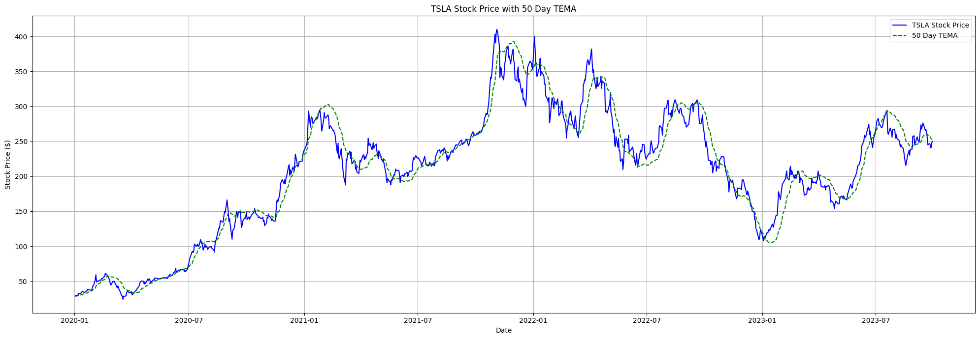
Part 1 — Fundamental Techniques: Simple Moving Average (SMA), Exponential Moving Average (EMA), Weighted Moving Average (WMA), Double Exponential Moving Average (DEMA), Triple Exponential Moving Average (TEMA), Volume Adjusted Moving Average (VAMA), Adaptive Moving Average (AMA or KAMA), Triangular Moving Average (TMA), Hull Moving Average (HMA)
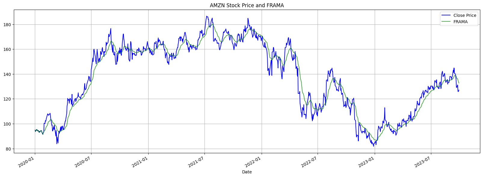
Part 2 — Adaptive and Dynamic: Fractal Adaptive Moving Average (FRAMA), Zero Lag Exponential Moving Average (ZLEMA), Variable Index Dynamic Average (VIDYA), Arnaud Legoux Moving Average (ALMA), MESA Adaptive Moving Average (MAMA), Following Adaptive Moving Average (FAMA) , Adaptive Period Moving Average, Rainbow Moving Average, Wilders Moving Average, Smoothed Moving Average (SMMA)
Part 3 — Advanced Weighting: Guppy Multiple Moving Average (GMMA), Least Squares Moving Average (LSMA), Welch’s Moving Average or Modified Moving Average, Sin-weighted Moving Average, Median Moving Average, Geometric Moving Average, Elastic Volume Weighted Moving Average (eVWMA), Regularized Exponential Moving Average (REMA), Parabolic Weighted Moving Average

Part 4 — From Niche to Noteworthy: Jurik Moving Average (JMA), End Point Moving Average (EPMA), Chande Moving Average (CMA), Harmonic Moving Average, McGinley Dynamic, Anchored Moving Average, Holt-Winters Moving Average, Filtered Moving Average, Kijun Sen (Base Line)
Good Credit Could Save You $200,000 Over Time

Better credit means better rates on mortgages, cars, and more. Cheers Credit Builder is an affordable, AI-powered way to start — no score or hard check required. We report to all three bureaus fast. Many users see 20+ point increases in months. Cancel anytime with no penalties or hidden fees.
2. Background and Python Implementation
This section explores the methodologies from both theoretical and practical standpoints. The ultimate goal is to offer a Python-based implementation to put them all to work.
2.1 Jurik Moving Average (JMA)
The Jurik Moving Average (JMA) was developed by Mark Jurik. It’s lauded for its smoothness and low lag, making it a favorite among traders. JMA aims to offer the best of both worlds by providing a smooth curve that closely tracks price action. The JMA is especially unique because it adjusts itself in real-time based on the volatility and price action.
The exact formula and calculation method for JMA is proprietary. However, there are approximations available, and many platforms provide the JMA as an inbuilt function. For our purposes, and to avoid any proprietary issues, I will not provide the exact formula but will provide a Python implementation based on available approximations and existing libraries.
While many moving averages require traders to compromise between responsiveness and smoothness, the JMA elegantly circumvents this dilemma. Its adaptive nature ensures that it remains closely tethered to current price movements, offering insights with reduced lag.
# Required Libraries
import yfinance as yf
import matplotlib.pyplot as plt
from pandas import Series
from numpy import average as npAverage
from numpy import nan as npNaN
from numpy import log as npLog
from numpy import power as npPower
from numpy import sqrt as npSqrt
from numpy import zeros_like as npZeroslike
from pandas_ta.utils import get_offset, verify_series

def jma(close, length=None, phase=None, offset=None, **kwargs):
    # Validate Arguments
    _length = int(length) if length and length > 0 else 7
    phase = float(phase) if phase and phase != 0 else 0
    close = verify_series(close, _length)
    offset = get_offset(offset)
    if close is None: return

    # Define base variables
    jma = npZeroslike(close)
    volty = npZeroslike(close)
    v_sum = npZeroslike(close)

    kv = det0 = det1 = ma2 = 0.0
    jma[0] = ma1 = uBand = lBand = close[0]

    # Static variables
    sum_length = 10
    length = 0.5 * (_length - 1)
    pr = 0.5 if phase < -100 else 2.5 if phase > 100 else 1.5 + phase * 0.01
    length1 = max((npLog(npSqrt(length)) / npLog(2.0)) + 2.0, 0)
    pow1 = max(length1 - 2.0, 0.5)
    length2 = length1 * npSqrt(length)
    bet = length2 / (length2 + 1)
    beta = 0.45 * (_length - 1) / (0.45 * (_length - 1) + 2.0)

    m = close.shape[0]
    for i in range(1, m):
        price = close[i]

        # Price volatility
        del1 = price - uBand
        del2 = price - lBand
        volty[i] = max(abs(del1),abs(del2)) if abs(del1)!=abs(del2) else 0

        # Relative price volatility factor
        v_sum[i] = v_sum[i - 1] + (volty[i] - volty[max(i - sum_length, 0)]) / sum_length
        avg_volty = npAverage(v_sum[max(i - 65, 0):i + 1])
        d_volty = 0 if avg_volty ==0 else volty[i] / avg_volty
        r_volty = max(1.0, min(npPower(length1, 1 / pow1), d_volty))

        # Jurik volatility bands
        pow2 = npPower(r_volty, pow1)
        kv = npPower(bet, npSqrt(pow2))
        uBand = price if (del1 > 0) else price - (kv * del1)
        lBand = price if (del2 < 0) else price - (kv * del2)

        # Jurik Dynamic Factor
        power = npPower(r_volty, pow1)
        alpha = npPower(beta, power)

        # 1st stage - prelimimary smoothing by adaptive EMA
        ma1 = ((1 - alpha) * price) + (alpha * ma1)

        # 2nd stage - one more prelimimary smoothing by Kalman filter
        det0 = ((price - ma1) * (1 - beta)) + (beta * det0)
        ma2 = ma1 + pr * det0

        # 3rd stage - final smoothing by unique Jurik adaptive filter
        det1 = ((ma2 - jma[i - 1]) * (1 - alpha) * (1 - alpha)) + (alpha * alpha * det1)
        jma[i] = jma[i-1] + det1

    # Remove initial lookback data and convert to pandas frame
    jma[0:_length - 1] = npNaN
    jma = Series(jma, index=close.index)

    # Offset
    if offset != 0:
        jma = jma.shift(offset)

    # Handle fills
    if "fillna" in kwargs:
        jma.fillna(kwargs["fillna"], inplace=True)
    if "fill_method" in kwargs:
        jma.fillna(method=kwargs["fill_method"], inplace=True)

    # Name & Category
    jma.name = f"JMA_{_length}_{phase}"
    jma.category = "overlap"

    return jma

# Fetch data
ticker_symbol = "AAPL"
data = yf.download(ticker_symbol, start="2020-01-01", end="2024-01-01")

# length
n = 28

# Compute JMA
data['JMA'] = jma(data['Close'], length=n, phase=0)

# Plot
plt.figure(figsize=(20,7))
plt.title(f'{ticker_symbol} Stock Price and JMA (n = {n})', fontsize=16)
plt.plot(data['Close'], label='Stock Price', color='black', alpha=0.6)
plt.plot(data['JMA'], label='JMA', color='green', alpha=0.8)
plt.legend(loc='upper left')
plt.grid(True, alpha=0.3)
plt.xlabel('Date', fontsize=14)
plt.ylabel('Price', fontsize=14)
plt.show()
Figure 1: Apple Inc. (AAPL) Stock Price from 2020 to 2023, complemented with the Jurik Moving Average (JMA) using a 14-day period and phase of 0. The JMA, known for its adaptive capabilities, provides an efficient smoothing of the price data while being responsive to market movements.
2.2 End Point Moving Average (EPMA)
The End Point Moving Average (EPMA) is a modified simple moving average that places more emphasis on the most recent data by calculating the linear regression trendline of the data set and using the end point of this trendline as the moving average.
The rationale is that this method will better capture the dominant trend in the price series and provide a more accurate representation than a simple moving average.
To compute the EPMA for a period n, the steps are:
Compute a linear regression trendline for the past n closing prices.
Use the endpoint of the regression line as the EPMA for that period.
The linear regression line’s formula is

Equation 2.2.1. Linear Regression: Used to calculate the trendline over a period ’n’ closing prices, which serves as the basis for the End Point Moving Average (EPMA).
Where:
m is the slope of the line.
xt is the x-coordinate of the time t (usually denoted as 1 for the first point, 2 for the second, and so on).
c is the y-intercept.

The best HR advice comes from those in the trenches. That’s what this is: real-world HR insights delivered in a newsletter from Hebba Youssef, a Chief People Officer who’s been there. Practical, real strategies with a dash of humor. Because HR shouldn’t be thankless—and you shouldn’t be alone in it.
The end point is when xt=n, so

Equation 2.2.2. EPMA: The y-coordinate of the linear regression line when xt=n. This endpoint provides a more focused representation of the current trend than a traditional SMA.
The EPMA aims to capture the essence of the current trend more effectively than the traditional SMA by focusing on the trend’s end point. It emphasizes the most recent data, potentially capturing the dominant market trend more effectively than traditional SMAs.
Its focus on the trend’s end point makes it especially valuable during volatile market phases, distinguishing genuine trend shifts from market noise. For traders, an upward-trending EPMA can signal bullish momentum, while a downward trend might hint at bearish conditions.
import yfinance as yf
import numpy as np
import matplotlib.pyplot as plt

def calculate_EPMA(prices, period):
    epma_values = []

    for i in range(period - 1, len(prices)):
        x = np.arange(period)
        y = prices[i-period+1:i+1]

        slope, intercept = np.polyfit(x, y, 1)
        epma = slope * (period - 1) + intercept

        epma_values.append(epma)

    return [None]*(period-1) + epma_values  # Pad with None for alignment

# Fetching data
ticker_symbol = "DIS"
data = yf.download(ticker_symbol, start="2020-01-01", end="2024-01-01")
close_prices = data['Close'].tolist()

# Calculate EPMA
epma_period = 28
data['EPMA'] = calculate_EPMA(close_prices, epma_period)

# Plotting
plt.figure(figsize=(20,7))
plt.plot(data.index, data['Close'], label=f'{ticker_symbol} Price', color='black')
plt.plot(data.index, data['EPMA'], label=f'EPMA {epma_period}', color='green')
plt.title(f'End Point Moving Average of {ticker_symbol} (n = {epma_period})')
plt.legend()
plt.grid()
plt.show()
Figure 2. End Point Moving Average (EPMA) of The Walt Disney Company (DIS) from 2020 to 2023: This graph shows DIS’s stock price (black line) and its 14-day EPMA (green line). The EPMA is calculated based on linear regression, providing a unique way to understand price trends.
2.3 Chande Moving Average (CMA)
The Chande Moving Average (CMA) is a type of moving average developed by Tushar Chande. It’s different from the common Simple Moving Average (SMA) because while the SMA considers only the closing prices in its calculation, the CMA considers all prices within the period to be equal. The Chande Moving Average sums up the cumulative prices and then divides by the cumulative number of prices.

Equation 2.3.1. Formula for the Chande Moving Average (CMA): Introduced by Tushar Chande, the CMA distinguishes itself from the conventional SMA by treating every price within its period as equal
Where:
CMA_t is the Chande Moving Average at time t.
Price_i is the price at time i.
In trading, the Chande Moving Average (CMA) offers a distinctive perspective on price movements, specifically addressing the potential biases of over-relying on closing prices. By giving equal weight to every price within its period, the CMA promotes a more holistic view of market activity. This inclusive approach can be particularly beneficial in markets with significant intra-day volatility or when closing prices might be susceptible to artificial manipulation or end-of-day trading anomalies.
For traders, using the CMA can provide a clearer picture of the underlying trend and reduce the likelihood of being misled by erratic price spikes or drops that don’t reflect the broader market sentiment. In essence, the CMA serves as a tool for a more democratically-informed trading decision, ensuring no single price point unduly influences the perceived trend.
import yfinance as yf
import numpy as np
import matplotlib.pyplot as plt

def calculate_CMA(prices):
    cumsum = np.cumsum(prices)
    cma = cumsum / (np.arange(len(prices)) + 1)
    return cma

# Fetching data
ticker_symbol = "KO"
data = yf.download(ticker_symbol, start="2020-01-01", end="2024-01-01")

# Calculate CMA
cma_period = len(data['Close'])
data['CMA'] = calculate_CMA(data['Close'])

# Plotting
plt.figure(figsize=(20,7))
plt.plot(data.index, data['Close'], label='Price', color='black')
plt.plot(data.index, data['CMA'], label='CMA', color='blue')
plt.title(f'Chande Moving Average (CMA) of {ticker_symbol}')
plt.legend()
plt.grid()
plt.show()
Figure 3. Chande Moving Average (CMA) of KO (2020–2023): The CMA is essentially the cumulative sum of closing prices divided by the number of days, hence it’s a moving average that considers all prior data. In the plot, Apple’s stock price (black) and its CMA (blue) are displayed. The CMA gives a smoothed representation of AAPL’s overall price trajectory since the start.
2.4 Harmonic Moving Average
The Harmonic Moving Average is a type of moving average that applies a harmonic mean formula. Unlike the arithmetic mean which averages the sum of values, the harmonic mean is the reciprocal of the arithmetic mean of the reciprocals.
It provides more weight to lower values than higher ones. Due to its unique calculation, the HMA may offer different insights into price trends, especially when prices exhibit specific patterns or rhythms.
Given a series of prices p1, p2,…, pn for n periods:

Equation 2.4.1. Fomrula for the Harmonic Moving Average (HMA): Utilizing the harmonic mean formula, the HMA emphasizes lower values over higher ones by applying the reciprocal of the arithmetic mean of the reciprocals.
For traders, the Harmonic Moving Average (HMA) presents an intriguing tool that emphasizes periods of lower prices, potentially highlighting buy opportunities or support levels more distinctly than other moving averages. This unique weighting can be especially useful in markets where price retracements and consolidations form essential parts of prevailing trends.
When applied alongside other indicators, the HMA can help identify periods of value or underpricing. Furthermore, in volatile markets where sudden price spikes might skew other averages, the HMA remains relatively stable, focusing more on consistent lower price points.
import yfinance as yf
import numpy as np
import matplotlib.pyplot as plt

def calculate_HMA(prices, window):
    hma_values = []
    for i in range(len(prices)):
        if i < window - 1:
            hma_values.append(np.nan)
        else:
            subset_prices = prices[i - window + 1: i + 1]
            harmonic_mean = window / np.sum([1/p for p in subset_prices])
            hma_values.append(harmonic_mean)
    return hma_values

# Fetching data
ticker_symbol = "MSFT"
data = yf.download(ticker_symbol, start="2020-01-01", end="2024-01-01")

# Calculate HMA
hma_period = 20
data['HMA'] = calculate_HMA(data['Close'], hma_period)

# Plotting
plt.figure(figsize=(20,7))
plt.plot(data.index, data['Close'], label='Price', color='black')
plt.plot(data.index, data['HMA'], label=f'HMA {hma_period}', color='blue')
plt.title(f'Harmonic Moving Average (HMA) of {ticker_symbol} (n = {hma_period})')
plt.legend()
plt.grid()
plt.show()
Figure 4. Harmonic Moving Average (HMA) of MSFT (2020–2023): The HMA is derived from the reciprocal of the arithmetic mean of the reciprocals of the previous n days’ closing prices. For this visualization, we’ve employed a 20-day window. The chart showcases Microsoft’s stock price (depicted in black) juxtaposed against its HMA (portrayed in blue). The HMA provides insights into the stock’s price trends by placing greater weight on values in the dataset that are more distant from the arithmetic mean, offering a distinctive perspective compared to traditional averages.
2.5 McGinley Dynamic
The McGinley Dynamic moving average was introduced by John R. McGinley in 1990. It is designed to be more responsive to the underlying data series than other moving averages. Its formula ensures that it tracks prices more closely during fast-moving markets and minimizes price separation during slower-moving markets. The goal is to avoid whipsaws while still reacting quickly to market trends.
The McGinley Dynamic is calculated as follows:

Equation 2.5.1. Formula for the McGinley Dynamic Moving Average: Introduced by John R. McGinley, this advanced moving average formula aims to track prices more effectively by minimizing lag in rapid markets and reducing separation during slower trends.
Where:
MD is the McGinley Dynamic value.
Price is the current price.
N is a constant (typically the same value you’d use for a moving average, such as 14 days for daily data).
In the trading world, the McGinley Dynamic offers a distinct advantage over traditional moving averages due to its self-adjusting mechanism. The calculation methodology inherently factors in the speed of market changes, allowing it to be more adaptive to real-time conditions.
This means traders can have greater confidence in the signals generated by the McGinley Dynamic, as it’s less likely to produce false signals or lag too far behind the price. Its unique behavior in tracking the asset price closely, regardless of market speed, can be a boon for traders aiming to exploit short-term price discrepancies.
import yfinance as yf
import matplotlib.pyplot as plt

def calculate_mcginley_dynamic(prices, n):
    MD = [prices[0]]
    for i in range(1, len(prices)):
        md_value = MD[-1] + (prices[i] - MD[-1]) / (n * (prices[i] / MD[-1])**4)
        MD.append(md_value)
    return MD

# Fetching data
ticker_symbol = "AAPL"
data = yf.download(ticker_symbol, start="2020-01-01", end="2024-01-01")

# Calculate McGinley Dynamic
n = 14
data['McGinley Dynamic'] = calculate_mcginley_dynamic(data['Close'].tolist(), n)

# Plotting
plt.figure(figsize=(20,7))
plt.plot(data.index, data['Close'], label='Price', color='black')
plt.plot(data.index, data['McGinley Dynamic'], label=f'McGinley Dynamic {n}', color='blue')
plt.title(f'McGinley Dynamic of {ticker_symbol} (n={n})')
plt.legend()
plt.grid()
plt.show()
Figure 5. McGinley Dynamic of AAPL (2020–2023): Designed to minimize lag, the McGinley Dynamic adapts to speed changes in Apple’s stock price. Displayed over a 14-day period, the chart contrasts Apple’s stock price (black) with its McGinley Dynamic (blue), showcasing a smoother representation of price movements.
2.6 Anchored Moving Average
The Anchored Moving Average (AMA) is a unique type of moving average that starts its calculation not from the first data point in a series but from a specific “anchored” point, typically a significant event date (e.g., a market bottom, breakout, news release, etc.). By anchoring the moving average, the emphasis is placed on the significance of that event and its continuing relevance to price action.
Formula:
The calculation of the AMA is essentially a Simple Moving Average (SMA) starting from the anchored date:

Equation 2.6.1. Formula for the Anchored Moving Average (AMA): The AMA places significance on a specific event in the data series by starting its calculation from that ‘anchored’ point.
Where:
AMAt is the Anchored Moving Average at time t.
Price denotes the price of the asset.
anchor is the anchored period.
The Anchored Moving Average, by emphasizing a specific event, offers traders a lens to view how prices evolve relative to that significant occurrence. Events like earnings announcements, regulatory changes, or macroeconomic data releases that can dramatically shift market sentiment, the AMA provides a persistent reminder of that event’s market impact. By focusing on the aftermath of such pivotal moments, traders can gain insights into the market’s perception of that event over time.
For instance, if prices consistently stay above the AMA after a positive earnings release, it indicates sustained bullish sentiment. Conversely, if prices drift below the AMA post a major news event, it can be a sign of prevailing bearish views. When used judiciously, the AMA can serve as a reference point, assisting traders in contextualizing recent price movements in light of past significant events.
import yfinance as yf
import matplotlib.pyplot as plt
from matplotlib.dates import date2num
from datetime import datetime

def calculate_AMA(prices, anchor_date):
    try:
        anchor_idx = data.index.get_loc(anchor_date)
    except KeyError:
        # If the exact date is not found, find the nearest available date
        anchor_date = data.index[data.index.get_loc(anchor_date, method='nearest')]
        anchor_idx = data.index.get_loc(anchor_date)

    AMA = []

    for i in range(len(prices)):
        if i < anchor_idx:
            AMA.append(None)
        else:
            AMA.append(sum(prices[anchor_idx:i+1]) / (i - anchor_idx + 1))

    return AMA
# Fetching data
ticker_symbol = "SIE.DE"
data = yf.download(ticker_symbol, start="2020-01-01", end="2024-01-01")

# Define the anchor date
anchor_date = "2021-01-01"
anchor_date_num = date2num(datetime.strptime(anchor_date, '%Y-%m-%d'))

# Calculate AMA
data['AMA'] = calculate_AMA(data['Close'].tolist(), anchor_date)

# Plotting
plt.figure(figsize=(20,7))
plt.plot(data.index, data['Close'], label='Price', color='black')
plt.plot(data.index, data['AMA'], label='Anchored MA', color='red')
plt.axvline(x=anchor_date_num, color='blue', linestyle='--', label='Anchor Date')
plt.title(f'Anchored Moving Average (AMA) of {ticker_symbol}')
plt.legend()
plt.grid()
plt.show()
Figure 6. Anchored Moving Average (AMA) of SAP.DE (2020–2023): The AMA begins calculation from a specific ‘anchor’ date, rather than a rolling window. It averages all data from this anchor point to the present. The plot showcases SAP’s stock price (black) juxtaposed with its AMA (red), starting from the blue dashed anchor date. The AMA provides insights into price trends since a significant event or chosen anchor date.
2.7 Holt-Winters Moving Average
The Holt-Winters method comprises three equations: one for the level, one for the trend, and one for the seasonality. Each equation has a smoothing parameter (alpha, beta, gamma) that controls the weight of the most recent observation.
Level — It’s the average value in the series.

Equation 2.7.1. Capturing the Average Value: The level (Lt) reflects the central tendency of the time series, indicating its average value. The smoothing parameter α determines the weight of the most recent observation.
Trend — It’s the increasing or decreasing value in the series.

Equation 2.7.2. Detecting Directional Changes: The trend (Tt) identifies the consistent upward or downward movement in the time series over time. It’s influenced by the smoothing parameter β, which considers the recent trend evolution.
Seasonality — It’s the repeating short-term cycle in the series.

Equation 2.7.3. Highlighting Short-Term Cycles: The seasonality (St) represents the periodic fluctuations that recur within fixed intervals, typically within a year. Its emphasis on recent cyclical patterns is governed by the smoothing parameter γ.
Forecast:

Equation 2.7.4. Projecting Future Values: This equation forecasts the future values of the time series using the identified level, trend, and seasonality. The parameter k specifies how many periods ahead the prediction extends.
Where:
Lt is the level at time t.
Tt is the trend at time t.
St is the seasonality at time t.
Yt is the actual value at time t.
m is the number of seasons.
α, β, γ are the smoothing parameters for level, trend, and seasonality, respectively.
k is the number of periods ahead you want to forecast.
What sets Holt-Winters apart from more rudimentary moving averages is its ability to adapt dynamically to changes in trend and seasonality. This adaptiveness is precisely why it’s favored in scenarios where time series data exhibits clear seasonal patterns, like retail sales that peak during holiday seasons or energy consumption that varies with seasons.
When applying Holt-Winters, traders and analysts should be judicious in tuning the smoothing parameters α, β, and γ. These parameters dictate how responsive the estimates are to recent changes in the level, trend, and seasonality of the series. By optimizing these parameters, one can strike a balance between responsiveness and smoothness.
import yfinance as yf
import matplotlib.pyplot as plt
from statsmodels.tsa.holtwinters import ExponentialSmoothing

# Fetching data
ticker_symbol = "INTC"
data = yf.download(ticker_symbol, start="2020-01-01", end="2024-01-01")

# Fit the Holt-Winters model
model = ExponentialSmoothing(data['Close'], trend='add', seasonal='add', seasonal_periods=12)
fit = model.fit()

# Calculate HWMA
data['HWMA'] = fit.fittedvalues

# Plotting
plt.figure(figsize=(20,7))
plt.plot(data.index, data['Close'], label='Price', color='black')
plt.plot(data.index, data['HWMA'], label='HWMA', color='red')
plt.title(f'Holt-Winters Moving Average (HWMA) of {ticker_symbol}')
plt.legend()
plt.grid()
plt.show()
Figure 7. Holt-Winters Moving Average (HWMA) of INTC (2020–2023): The HWMA (red) applies exponential smoothing techniques, considering both trend and seasonality, to depict INTC’s stock price movement. Displayed against the actual closing price (black), it provides insights into the underlying trend and potential seasonality in the stock’s performance.
2.8 Filtered Moving Average
The concept behind the Filtered Moving Average is to use a filter mechanism (like a digital or analog filter) to eliminate certain frequencies from the data set. This helps to emphasize specific frequency bands (for example, trends) while removing noise.
The FMA is defined as:

Equation 2.8.1. Emphasizing Trends, Reducing Noise: The Filtered Moving Average (FMA) integrates a filter mechanism to prioritize certain frequencies, allowing it to accentuate specific trends and diminish unwanted noise. The weights w(i) applied are determined by the type of filter chosen, while n denotes the moving average period.
Where:
P(t−i) is the price at time t−i.
w(i) is the weight for the price at time t−i. The specific weights depend on the filter applied.
n is the period of the moving average.
The Filtered Moving Average (FMA) is designed to emphasize specific frequency bands within a dataset, effectively enhancing the clarity of underlying trends and reducing the impact of short-term fluctuations. This method offers an analytical edge by mitigating the effects of market noise, which can obscure genuine market movements.
The FMA’s emphasis on prioritized frequencies can assist in distinguishing real shifts in market sentiment from transient market events. The effectiveness of the FMA relies on the selection of an appropriate filter and the correct period (n). By refining these parameters to match the specific nature of the dataset and the strategic objectives, the FMA can provide more precise and actionable insights into market dynamics.
import yfinance as yf
import numpy as np
import matplotlib.pyplot as plt

def filtered_moving_average(prices, n=14):
    # Define filter weights (for simplicity, we'll use equal weights similar to SMA)
    w = np.ones(n) / n
    return np.convolve(prices, w, mode='valid')

# Fetching data
ticker_symbol = "MCD"
data = yf.download(ticker_symbol, start="2020-01-01", end="2024-01-01")

fma_period = 14
fma_values = filtered_moving_average(data['Close'].values, fma_period)
data['FMA'] = np.concatenate([np.array([np.nan]*(fma_period-1)), fma_values])

# Plotting
plt.figure(figsize=(20,7))
plt.plot(data.index, data['Close'], label='Price', color='black')
plt.plot(data.index, data['FMA'], label=f'Filtered MA {fma_period}', color='red')
plt.title(f'Filtered Moving Average (FMA) of {ticker_symbol} (n = {fma_period})')
plt.legend()
plt.grid()
plt.show()
Figure 8. Filtered Moving Average (FMA) of MCD (2020–2023): The FMA (red) is essentially a simple moving average that has been enhanced by using a filter (in this case, a simple equal weight filter) to better emphasize certain data characteristics. When plotted against the actual closing price (black) of McDonald’s stock, the FMA provides a smoother representation of price trends over the given period, making it easier to discern underlying patterns and movements. The choice of filter can be adjusted to emphasize specific patterns or characteristics in the data.
2.9 Kijun Sen (Base Line)
The Kijun Sen, also known as the Base Line, represents the midpoint of the highest high and the lowest low over a certain period, commonly 26 periods. In the Ichimoku Cloud setup, the Kijun Sen serves multiple purposes:
Trend Indicator: If the price is above the Kijun Sen, it indicates an uptrend, and if it’s below the Kijun Sen, it suggests a downtrend.
Support and Resistance: The Kijun Sen acts as a dynamic level of support and resistance.
Signal for Buy or Sell: When the faster-moving Tenkan Sen (Conversion Line) crosses above the Kijun Sen, it’s considered a bullish signal, and when it crosses below, it’s a bearish signal.

Equation 2.9.1. The Kijun Sen or Base Line represents the equilibrium between the highest high and the lowest low over a typically chosen 26-period span
The Kijun Sen, an integral component of the Ichimoku Cloud trading system, holds substantial importance in technical analysis due to its multifunctional attributes. Being calculated as the midpoint of a selected time frame’s highest high and lowest low, it inherently possesses a self-adjusting nature, reflecting market equilibrium and a clear barometer for market sentiment.
Furthermore, as it acts dynamically to price movements, its ability to offer real-time support and resistance levels can be vital for entry and exit decisions. Strategically, recognizing intersections between the Kijun Sen and Tenkan Sen can assist in pinpointing momentum shifts, thereby guiding trading strategies.
import yfinance as yf
import numpy as np
import matplotlib.pyplot as plt

def calculate_kijun_sen(data, period=26):
    # Determine the highest high and the lowest low for the given period
    high_prices = data['High'].rolling(window=period).max()
    low_prices = data['Low'].rolling(window=period).min()

    # Calculate Kijun Sen (Base Line)
    kijun_sen = (high_prices + low_prices) / 2
    return kijun_sen

# Fetching data
ticker_symbol = "WMT"
data = yf.download(ticker_symbol, start="2020-01-01", end="2024-01-01")

# Calculate Kijun Sen
data['Kijun Sen'] = calculate_kijun_sen(data)

# Plotting
plt.figure(figsize=(20,7))
plt.plot(data.index, data['Close'], label='Price', color='black')
plt.plot(data.index, data['Kijun Sen'], label='Kijun Sen (Base Line)', color='blue')
plt.title(f'Kijun Sen (Base Line) of {ticker_symbol}')
plt.legend()
plt.grid()
plt.show()
Figure 9. Kijun Sen (Base Line) of AAPL (2020–2023): The Kijun Sen (blue) represents the equilibrium point between the highest high and the lowest low over a typical span of 26 periods. When plotted against the actual closing price (black) of Apple’s stock, the Kijun Sen serves as a dynamic reference line. Being above the Kijun Sen may suggest an uptrend, while being below can indicate a potential downtrend.
3. Applications & Insights
Niche moving average techniques offer traders unique perspectives on the market, challenging them to think beyond traditional paradigms. The McGinley Dynamic moving average, for instance, promises to be the most reliable moving average, underscoring the pursuit of accuracy in trading.
The Holt-Winters moving average, on the other hand, offers a forecasted approach, assisting in predictive analytics. It uses a combination of exponential smoothing and seasonal adjustments to generate forecasts of future price movements. This makes it a valuable tool for traders who are looking to identify and exploit market trends.
Here are a few specific examples of how niche moving average techniques can be used in trading:
The McGinley Dynamic moving average can be used to identify trends and reversals. It is also useful for identifying support and resistance levels.
The Holt-Winters moving average can be used to generate forecasts of future price movements. It can also be used to identify seasonal patterns in the market.
4. Concluding Thoughts
Every trader equips themselves with a set of techniques, and while conventional tools lay the foundation, niche moving averages often fine-tune a strategy to get closer to perfection. These specialized averages excel in volatile markets due to their adaptability and reduced susceptibility to false signals, offering unique market insights. However, they come with complexities: intricate calculations and parameter settings.
For those ready to delve deep, these niche techniques promise enhanced market comprehension, better strategy formulation, and refined risk management. Yet, they aren’t a guaranteed recipe for success. Their real potential is unlocked when coupled with a sound strategy, emotional discipline, and robust risk management.
Subscribe to our premium content to read the rest.
Become a paying subscriber to get access to this post and other subscriber-only content.
Upgrade