
In partnership with

Become An AI Expert In Just 5 Minutes

If you’re a decision maker at your company, you need to be on the bleeding edge of, well, everything. But before you go signing up for seminars, conferences, lunch ‘n learns, and all that jazz, just know there’s a far better (and simpler) way: Subscribing to The Deep View.
This daily newsletter condenses everything you need to know about the latest and greatest AI developments into a 5-minute read. Squeeze it into your morning coffee break and before you know it, you’ll be an expert too.
Subscribe right here. It’s totally free, wildly informative, and trusted by 600,000+ readers at Google, Meta, Microsoft, and beyond.
🔔 Limited-Time Holiday Deal: 20% Off Our Complete 2026 Playbook! 🔔
Level up before the year ends!
AlgoEdge Insights: 30+ Python-Powered Trading Strategies – The Complete 2026 Playbook
30+ battle-tested algorithmic trading strategies from the AlgoEdge Insights newsletter – fully coded in Python, backtested, and ready to deploy. Your full arsenal for dominating 2026 markets.
Special Promo: Use code DECEMBER2025 for 20% off
Valid only until February 20, 2026 — act fast!
👇 Buy Now & Save 👇

Instant access to every strategy we've shared, plus exclusive extras.
— AlgoEdge Insights Team
🔔 Flash Launch Alert: AlgoEdge Colab Vault – Your 2026 Trading Edge! 🔔
I've turned my 20 must-have, battle-tested Python strategies into fully executable Google Colab notebooks – ready to run in your browser with one click.

One-click notebooks • Real-time data • Bias-free backtests • Interactive charts • OOS tests • CSV exports • Pro metrics
Test on any ticker instantly (SPY, BTC, PLTR, TSLA, etc.).
Launch Deal (ends Feb 28, 2026):
$129 one-time (save $40 – regular $169 after)
Lifetime access + free 2026 updates.
Inside the Vault (20 powerhouses):
Bias-Free Cubic Poly Trend
3-State HMM Volatility Filter
MACD-RSI Momentum
Bollinger Squeeze Breakout
Supertrend ATR Rider
Ichimoku Cloud
VWAP Scalper
Donchian Breakout
Keltner Reversion
RSI Divergence
MA Ribbon Filter
Kalman Adaptive Trend
ARIMA-GARCH Vol Forecast
LSTM Predictor
Random Forest Regime Classifier
Pairs Cointegration
Monte Carlo Simulator
FinBERT Sentiment
Straddle IV Crush
Fibonacci Retracement
👇 Grab It Before Price Jumps 👇
Buy Now – $129
P.S. Run code today → test live tomorrow → outperform the book readers.
Premium Members – Your Full Notebook Is Ready
The complete Google Colab notebook from today’s article (with live data, full Hidden Markov Model, interactive charts, statistics, and one-click CSV export) is waiting for you.
Preview of what you’ll get:

Inside:
Complete Part 1 collection — all 9 fundamental moving average techniques from the popular "36 Moving Average Methods" series in one single Colab cell
Ready-to-run code for:
Simple Moving Average (SMA) – example with AAPL
Exponential Moving Average (EMA) – example with MSFT
Weighted Moving Average (WMA) – example with META
Double Exponential Moving Average (DEMA) – example with ASML
Triple Exponential Moving Average (TEMA) – example with TSLA
Volume Adjusted Moving Average (VAMA / VWMA style) – example with NVDA
Kaufman’s Adaptive Moving Average (KAMA / AMA) – example with BRK-B
Triangular Moving Average (TMA) – example with GOOGL
Hull Moving Average (HMA) – example with JPM (includes custom helper functions)
Each method plotted beautifully next to real historical price data (2020–2023 by default)
Clean, well-commented Python code using yfinance + pandas + matplotlib
Easy to customize: change tickers, periods, date ranges, or add your own stocks in seconds
All imports and setup in one place — just Run → All and watch the charts appear
Great starting point to experiment with crossovers, multiple MAs on one chart, or extend to Parts 2–4 later
Perfect for learning, backtesting ideas, or quickly visualizing how different moving averages behave in real markets
Free readers – you already got the full breakdown and visuals in the article. Paid members – you get the actual tool.
Not upgraded yet? Fix that in 10 seconds here👇
Google Collab Notebook With Full Code Is Available In the End Of The Article Behind The Paywall 👇 (For Paid Subs Only)
1. Introduction
Moving averages are one of the most widely used technical indicators by traders and investors of all levels. They help to smooth out the inherent volatility of stock prices by calculating the average price over a specified period. Moving averages can be simple to calculate, but there are also more complex forms that are designed to capture more nuance aspects of the market.
This four-part series will discuss a total of 36 different moving average methods, from the foundational to the more sophisticated and niche. We will cover the methodology and implementation of each method, and provide the Python code for you to plug and play. Given the signficant amount of methods, we’ve grouped them as follows:
Part 1 — Fundamental Techniques: Simple Moving Average (SMA), Exponential Moving Average (EMA), Weighted Moving Average (WMA), Double Exponential Moving Average (DEMA), Triple Exponential Moving Average (TEMA), Volume Adjusted Moving Average (VAMA), Adaptive Moving Average (AMA or KAMA), Triangular Moving Average (TMA), Hull Moving Average (HMA)
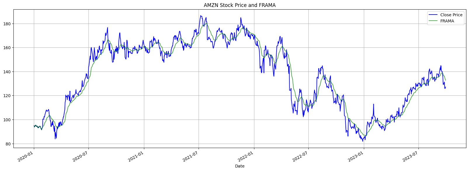
Part 2— Adaptive and Dynamic: Fractal Adaptive Moving Average (FRAMA), Zero Lag Exponential Moving Average (ZLEMA), Variable Index Dynamic Average (VIDYA), Arnaud Legoux Moving Average (ALMA), MESA Adaptive Moving Average (MAMA), Following Adaptive Moving Average (FAMA) , Adaptive Period Moving Average, Rainbow Moving Average, Wilders Moving Average, Smoothed Moving Average (SMMA)
The 1 part is free for all my subscribers, however the second part is available only for paid subs
2. Background and Python Implementation
This section explores the methodologies from both theoretical and practical standpoints. The ultimate goal is to offer a Python-based implementation to put them all to work.
Billionaire investors just set 2 all-time records. An asset class most investors never even considered.

How have 70,679 everyday investors joined in on the billionaire’s asset class?
A Klimt painting sold for $236 million—the most expensive modern artwork ever sold at auction.
A Kahlo broke the auction record for a female artist at $54 million.
Obvious outliers, sure, but the 2025 fall auction season signaled the postwar and contemporary art market could be entering a bull run.
Why?
Outpaced the S&P 500 overall with low correlation since ‘95*
Can trade in any global currency
Natural scarcity
Of course, who can afford to spend millions on a painting, right?
But now it’s easy to fractionally invest in art by legends like Banksy and more, thanks to Masterworks.
They acquire it, securitize it, offer shares, and eventually look to sell it.
Net annualized returns like 14.6%, 17.6%, and 17.8% for works held over a year.
See why members have allocated $1.3 billion across 500+ works:
*According to Masterworks data. Investing involves risk. Past performance not indicative of future returns. See important disclosures at masterworks.com/cd.
2.1 Simple Moving Average (SMA)
The Simple Moving Average, commonly referred to as SMA, is one of the most basic and commonly used technical analysis tools. At its core, the SMA calculates the average price of a security over a set number of periods.
This average smoothens out short-term price fluctuations, allowing traders to understand the underlying trend of the stock. The longer the period chosen for the SMA, the smoother the curve; however, it might also lag behind the actual price movements.

Equation 2.1.1. Mathematical Representation of the Simple Moving Average (SMA) for a Defined Period.
When a stock price exceeds its SMA, it’s typically seen as a bullish sign, indicating potential upward movement. Conversely, falling below the SMA suggests a possible downtrend.
The “crossover” strategy is also prevalent, where traders observe a short and long-term SMA. A bullish sign is noted when the short-term crosses above the long-term, and vice versa for a bearish signal.
# Required Libraries
import yfinance as yf
import matplotlib.pyplot as plt
import pandas as pd

# Fetch data
ticker_symbol = "AAPL"
data = yf.download(ticker_symbol, start="2020-01-01", end="2024-01-01")

# Calculate SMA
sma_period = 50  # Example: 50 days SMA
data['SMA'] = data['Close'].rolling(window=sma_period).mean()

# Plot
plt.figure(figsize=(20,7))
plt.plot(data['Close'], label=f'{ticker_symbol} Stock Price', color='blue')
plt.plot(data['SMA'], label=f'{sma_period} Day SMA', color='red', linestyle='--')
plt.title(f'{ticker_symbol} Stock Price with 50 Day SMA (n={sma_period})')
plt.xlabel('Date')
plt.ylabel('Stock Price')
plt.legend()
plt.grid(True)
plt.tight_layout()
plt.show()
Figure 1. Apple Inc. (AAPL) Stock Price and its 50-Day Simple Moving Average (SMA) from 2020 to 2023.
2.2 Exponential Moving Average (EMA)
The Exponential Moving Average (EMA) is another vital tool in technical analysis, but unlike the SMA, it gives more weight to the most recent prices. This weighting provides the EMA with a slight advantage over the SMA, as it reacts more quickly to price changes.
The primary benefit of the EMA is its sensitivity, making it a preferred choice when determining short-term price movements and potential market entry and exit points.

Equation 2.2.1 Formula for the Exponential Moving Average (EMA) with Smoothing Factor α.
EMAt is the Exponential Moving Average for the current time t
Pt is the price for the current time t
α is the smoothing factor, calculated as α = 2 / (N+1)
N is the period of the EMA
EMAt−1 is the Exponential Moving Average for the previous time t−1
The EMA’s rapid reaction to price fluctuations is both its strength and challenge. Its heightened sensitivity provides quick insights, making it invaluable for tracking short-term market movements.
However, this very trait can sometimes amplify the effects of short-term volatility, potentially leading to reactive or mistimed trades.
# Required Libraries
import yfinance as yf
import matplotlib.pyplot as plt
import pandas as pd

# Fetch data
ticker_symbol = "MSFT"
data = yf.download(ticker_symbol, start="2020-01-01", end="2024-01-01")

# Calculate EMA
ema_period = 50
data['EMA'] = data['Close'].ewm(span=ema_period, adjust=False).mean()

# Plot
plt.figure(figsize=(20,7))
plt.plot(data['Close'], label=f'{ticker_symbol} Stock Price', color='blue')
plt.plot(data['EMA'], label=f'50 Day EMA', color='green', linestyle='--')
plt.title(f'{ticker_symbol} Stock Price with 50 Day EMA')
plt.xlabel('Date')
plt.ylabel('Stock Price')
plt.legend()
plt.grid(True)
plt.tight_layout()
plt.show()
Figure 2. Microsoft Corporation (MSFT) Stock Price and its 50-Day Exponential Moving Average (EMA) from 2020 to 2023.
2.3 Weighted Moving Average (WMA)
The Weighted Moving Average (WMA) assigns a weight to each data point based on its age. Unlike the SMA which gives equal weight to all data points, the WMA gives more importance to the recent prices, and less importance to older prices.
Essentially, this method allows traders to highlight recent movements in prices over older ones, capturing potential trends earlier than the SMA. The WMA is commonly used for short-term price forecasting.
The WMA is calculated using the following formula:

Equation 2.3.1. Mathematical Expression for the Weighted Moving Average (WMA) with Defined Weights.
Pi is the price for the ith period.
wi is the weight assigned to the price for the ith period.
N is the period of the WMA.
Typically, weights decrease linearly. For example, for a 3-day WMA, the most recent day’s price might be multiplied by 3, the previous day by 2, and the oldest day by 1.
The nuanced weighting mechanism of the WMA provides a distinctive edge in capturing emerging market trends. Its design inherently leans into recent market activities.
However, this very emphasis on recent data means the WMA might be more susceptible to short-term market noise or volatility. For traders who prioritize recent market actions, the WMA can be a potent asset.
# Required Libraries
import yfinance as yf
import matplotlib.pyplot as plt
import pandas as pd
import numpy as np

# Fetch data
ticker_symbol = "META"
data = yf.download(ticker_symbol, start="2020-01-01", end="2024-01-01")

# Calculate WMA
wma_period = 50  # Example: 50 days WMA
weights = np.arange(1, wma_period + 1)
data['WMA'] = data['Close'].rolling(window=wma_period).apply(lambda prices: np.dot(prices, weights)/weights.sum(), raw=True)

# Plot
plt.figure(figsize=(20,7))
plt.plot(data['Close'], label=f'{ticker_symbol} Stock Price', color='blue')
plt.plot(data['WMA'], label=f'{wma_period} Day WMA', color='orange', linestyle='--')
plt.title(f'{ticker_symbol} Stock Price with {wma_period} Day WMA')
plt.xlabel('Date')
plt.ylabel('Stock Price')
plt.legend()
plt.grid(True)
plt.tight_layout()
plt.show()
Figure 3. Meta Platforms, Inc. (META) Stock Price with its 50-Day Weighted Moving Average (WMA) from 2020 to 2023, showcasing the dynamic weighting emphasis on recent prices.
2.4 Double Exponential Moving Average (DEMA)
The Double Exponential Moving Average (DEMA) is a refinement of the traditional EMA, designed to be more responsive to recent price changes. It’s an attempt to reduce the lag inherent in simple moving averages or even EMAs.
The DEMA does this by taking the difference between a single EMA and a double EMA and adding it back to the original EMA. Because of this, DEMA reacts more quickly to price changes than the traditional EMA.

Most coverage tells you what happened. Fintech Takes is the free newsletter that tells you why it matters. Each week, I break down the trends, deals, and regulatory shifts shaping the industry — minus the spin. Clear analysis, smart context, and a little humor so you actually enjoy reading it. Subscribe free.
Calculate the EMA over period N

Equation 2.4.1. Exponential Moving Average (EMA) for a period of N day.
2. Calculate the EMA of EMA_N over the same period

Equation 2.4.2. Exponential Moving Average of the first EMA, both spanning N days.
3. The DEMA is given by:

Equation 2.4.3. Formulation of the Double Exponential Moving Average (DEMA) for Enhanced Trend Sensitivity.
Where:
P is the price for the current period.
α is the smoothing constant, and it’s equal to 2 / (N+1)
The DEMA’s heightened responsiveness makes it particularly appealing for traders who wish to act on swift market changes. When prices exhibit rapid fluctuations, the DEMA is more adept at highlighting emerging trends or reversals, potentially offering a trader an advantageous entry or exit point. This becomes especially valuable in volatile markets where timeliness can make a significant difference.
# Required Libraries
import yfinance as yf
import matplotlib.pyplot as plt
import pandas as pd

# Fetch data
ticker_symbol = "ASML"
data = yf.download(ticker_symbol, start="2020-01-01", end="2024-01-01")

# Calculate DEMA
dema_period = 50
alpha = 2 / (dema_period + 1)
data['EMA'] = data['Close'].ewm(span=dema_period, adjust=False).mean()
data['EMA2'] = data['EMA'].ewm(span=dema_period, adjust=False).mean()
data['DEMA'] = 2 * data['EMA'] - data['EMA2']

# Plot
plt.figure(figsize=(20,7))
plt.plot(data['Close'], label=f'{ticker_symbol} Stock Price', color='blue')
plt.plot(data['DEMA'], label=f'{dema_period} Day DEMA', color='red', linestyle='--')
plt.title(f'{ticker_symbol} Stock Price with {dema_period} Day DEMA')
plt.xlabel('Date')
plt.ylabel('Stock Price')
plt.legend()
plt.grid(True)
plt.tight_layout()
plt.show()
Figure 4. ASML Holding N.V. (ASML) Stock Price plotted against its 50-Day Double Exponential Moving Average (DEMA) from 2020 to 2023, illustrating DEMA’s enhanced responsiveness to price changes.
2.5 Triple Exponential Moving Average (TEMA)
The Triple Exponential Moving Average (TEMA) is another enhancement of the EMA. It aims to further reduce the lag and noise associated with single and double EMAs.
TEMA essentially triples the weighting of recent prices to become even more sensitive to price changes. It’s calculated using three EMAs: a single EMA, a double EMA (DEMA), and a triple EMA. By subtracting out the “lagged” effects of the first two, TEMA becomes highly responsive.
Calculate the EMA over period N

Equation 2.5.1. Exponential Moving Average (EMA) for a period of N days.
2. Calculate the EMA of EMA_N over the same period

Equation 2.5.2. Secondary Exponential Moving Average calculated from the EMA of period N days.
3. Calculate the EMA of EMA_N,2 over the same period

Equation 2.5.3. Tertiary Exponential Moving Average derived from the second EMA of period N days.
4. The TEMA is then given by:

Equation 2.5.4. Triple Exponential Moving Average (TEMA) combining the three EMAs.
Where:
P is the price for the current period.
α is the smoothing constant, and it’s equal to 2/(N+1)
By tripling down on recent price movements, TEMA stands out as a tool finely tuned to the market’s immediate dynamics. This makes it invaluable in volatile trading conditions where capturing subtle shifts is crucial. Yet, its sharp sensitivity can also elevate the risk of overvaluing fleeting price deviations. As a result, traders using TEMA must exercise discernment to distinguish authentic market movements from transient anomalies.
# Required Libraries
import yfinance as yf
import matplotlib.pyplot as plt
import pandas as pd

# Fetch data
ticker_symbol = "TSLA"
data = yf.download(ticker_symbol, start="2020-01-01", end="2024-01-01")

# Calculate TEMA
tema_period = 50
alpha = 2 / (tema_period + 1)
data['EMA'] = data['Close'].ewm(span=tema_period, adjust=False).mean()
data['EMA2'] = data['EMA'].ewm(span=tema_period, adjust=False).mean()
data['EMA3'] = data['EMA2'].ewm(span=tema_period, adjust=False).mean()
data['TEMA'] = 3 * data['EMA'] - 3 * data['EMA2'] + data['EMA3']

# Plot
plt.figure(figsize=(20,7))
plt.plot(data['Close'], label=f'{ticker_symbol} Stock Price', color='blue')
plt.plot(data['TEMA'], label=f'{tema_period} Day TEMA', color='green', linestyle='--')
plt.title(f'{ticker_symbol} Stock Price with {tema_period} Day TEMA')
plt.xlabel('Date')
plt.ylabel('Stock Price')
plt.legend()
plt.grid(True)
plt.tight_layout()
plt.show()
Figure 5. Tesla, Inc. (TSLA) Stock Price with its 50-Day Triple Exponential Moving Average (TEMA) from 2020 to 2023, showcasing TEMA’s advanced filtering of price noise.
2.6 Volume Adjusted Moving Average (VAMA)
The Volume Adjusted Moving Average (VAMA) integrates volume data into the moving average calculation, thereby giving more importance to prices that are accompanied by higher volume.
This means that during periods of higher trading activity, the VAMA will give more weight to the current price, making it more responsive. VAMA can be especially useful in identifying the strength of price movements, as large moves backed by substantial volume might be more sustainable.

Equation 2.6.1. Volume Adjusted Moving Average (VAMA) accounting for the significance of volume in price movements over a specified period N.
Where:
Pi is the closing price for period i.
Vi is the trading volume for period i.
N is the specified number of periods.
When a significant price change is backed by high volume, it often signals a stronger consensus among traders about the asset’s value, making VAMA particularly adept at highlighting robust trends.
One of the main criticisms of VAMA is that it may not respond as quickly to changes in price and volume. Since EVWMA addresses this shortcoming by placing a larger weight on recent data (both in terms of price and volume), therefore, being more reactive to recent market events. EVWMA is further discussed in article 3 of this series.
# Required Libraries
import yfinance as yf
import matplotlib.pyplot as plt
import pandas as pd

# Fetch data
ticker_symbol = "NVDA"
data = yf.download(ticker_symbol, start="2020-01-01", end="2024-01-01")

# Calculate VAMA
vama_period = 50
data['Volume_Price'] = data['Close'] * data['Volume']
data['VAMA'] = data['Volume_Price'].rolling(window=vama_period).sum() / data['Volume'].rolling(window=vama_period).sum()

# Plot
plt.figure(figsize=(20,7))
plt.plot(data['Close'], label=f'{ticker_symbol} Stock Price', color='blue')
plt.plot(data['VAMA'], label=f'{vama_period} Day VAMA', color='orange', linestyle='--')
plt.title(f'{ticker_symbol} Stock Price with {vama_period} Day VAMA')
plt.xlabel('Date')
plt.ylabel('Stock Price')
plt.legend()
plt.grid(True)
plt.tight_layout()
plt.show()
Figure 6. NVIDIA Corporation (NVDA) Stock Price compared with its 50-Day Volume-Adjusted Moving Average (VAMA) from 2020 to 2023, emphasizing the influence of trading volume on price movement.
2.7 Adaptive Moving Average (AMA or KAMA)
KAMA was developed by Perry Kaufman and is designed to be more responsive to price changes compared to other moving averages. The key feature of KAMA is its adaptability: it adjusts the smoothing constant based on the market’s volatility.
When the price moves in a strong trend, KAMA becomes more sensitive, and during range-bound, sideways market conditions, KAMA becomes smoother to filter out noise.
This adaptability is achieved through the Efficiency Ratio (ER), which measures the price directionality and volatility, and the Smoothing Constant (SC), which is derived from the ER and defines the weight given to the most recent price data.

Equation 2.7.1. Efficiency Ratio (ER) representing the price change rate relative to its volatility.

Equation 2.7.2. Determination of the Smoothing Constant (SC) using the Efficiency Ratio, fastest SC, and slowest SC.

Equation 2.7.3. Calculation of Kaufman’s Adaptive Moving Average (KAMA) by incorporating the dynamic Smoothing Constant.
Where:
ER is the Efficiency Ratio.
SC is the Smoothing Constant.
The fastest SC and the slowest SC are typically set at 2/(2+1) and 2/(30+1) respectively.
By dynamically adjusting its sensitivity based on market volatility, KAMA offers traders a unique blend of responsiveness and stability. During times of pronounced price trends, KAMA intensifies its sensitivity, enabling traders to pinpoint potential breakout or breakdown scenarios.
On the other hand, in more subdued, lateral market phases, KAMA showcases its versatility by tempering responses to trivial price shifts, thereby lessening the likelihood of misleading indicators.
# Required Libraries
import yfinance as yf
import matplotlib.pyplot as plt
import pandas as pd

# Fetch data
ticker_symbol = "BRK-B"
data = yf.download(ticker_symbol, start="2020-01-01", end="2024-01-01")

# Calculate KAMA
n = 10
fastest_SC = 2 / (2 + 1)
slowest_SC = 2 / (30 + 1)

data['Change'] = abs(data['Close'] - data['Close'].shift(n))
data['Volatility'] = data['Close'].diff().abs().rolling(window=n).sum()

data['ER'] = data['Change'] / data['Volatility']
data['SC'] = (data['ER'] * (fastest_SC - slowest_SC) + slowest_SC)**2

data['KAMA'] = data['Close'].copy()
for i in range(n, len(data)):
    data['KAMA'].iloc[i] = data['KAMA'].iloc[i-1] + data['SC'].iloc[i] * (data['Close'].iloc[i] - data['KAMA'].iloc[i-1])

# Plot
plt.figure(figsize=(20,7))
plt.plot(data['Close'], label=f'{ticker_symbol} Stock Price', color='blue')
plt.plot(data['KAMA'], label=f'KAMA (n={n})', color='green', linestyle='--')
plt.title(f'{ticker_symbol} Stock Price with KAMA (n={n})')
plt.xlabel('Date')
plt.ylabel('Stock Price')
plt.legend()
plt.grid(True)
plt.tight_layout()
plt.show()
Figure 7. Berkshire Hathaway Inc. Class B (BRK-B) Stock Price with its Kaufman’s Adaptive Moving Average (KAMA) from 2020 to 2023, illustrating the adaptive nature of KAMA based on price volatility.
2.8 Triangular Moving Average (TMA)
The Triangular Moving Average is a type of smoothed moving average that puts the most weight on the middle prices of the dataset. It’s essentially an average of an average, providing a smoothing effect that’s more profound than the Simple Moving Average.
Due to the added smoothing, the TMA can lag behind price more than other moving averages, but this can be advantageous when trying to eliminate insignificant price fluctuations.

Equation 2.8.1. Calculation of the Triangular Moving Average (TMA) emphasizing the central prices by using a weighted Simple Moving Average (SMA).
SMA(t, n+1/2 ) is the SMA at time t over n+1/2 periods.
t is the current period.
n is the number of periods chosen for the TMA.
The Triangular Moving Average offers traders a uniquely smoothed perspective on price trends. Its double-layered averaging process filters out the short-term market noise more efficiently than the Simple Moving Average.
This deliberate lag is TMA’s strength when traders aim to sidestep inconsequential price movements and focus on overarching trends. However, the very quality that makes TMA a formidable noise reducer can also cause it to react slower to genuine market shifts.
# Required Libraries
import yfinance as yf
import matplotlib.pyplot as plt
import pandas as pd

# Fetch data
ticker_symbol = "GOOGL"
data = yf.download(ticker_symbol, start="2020-01-01", end="2024-01-01")

# Calculate TMA
n = 20
half_n = (n+1) // 2
data['Half_SMA'] = data['Close'].rolling(window=half_n).mean()
data['TMA'] = data['Half_SMA'].rolling(window=half_n).mean()

# Plot
plt.figure(figsize=(20,7))
plt.plot(data['Close'], label=f'{ticker_symbol} Stock Price', color='blue')
plt.plot(data['TMA'], label=f'TMA (n={n})', color='red', linestyle='--')
plt.title(f'{ticker_symbol} Stock Price with TMA (n={n})')
plt.xlabel('Date')
plt.ylabel('Stock Price')
plt.legend()
plt.grid(True)
plt.tight_layout()
plt.show()
Figure 8. Alphabet Inc. (GOOGL) Stock Price alongside its Triangular Moving Average (TMA) from 2020 to 2023, showcasing the profound smoothing effect of the TMA on the stock’s price movements.
2.9 Hull Moving Average (HMA)
The Hull Moving Average is designed to eliminate lag and improve smoothing, making it responsive to current prices. Alan Hull developed this average to keep up with price action while maintaining a curve that’s smooth.
By taking the weighted average of the SMA, and then further smoothing it, HMA minimizes the lag of traditional moving averages while emphasizing recent prices. Below are the steps to calculate HMA:
Calculate a Weighted Moving Average with period n / 2 (which is just half of the period you want to use).
Calculate a Weighted Moving Average for period n.
Calculate the sqrt(n) weighted moving average of the difference between the two averages (from step 1 and 2).

Equation 2.9.1. Steps and formulas for calculating the Hull Moving Average (HMA), designed to provide a responsive yet smooth representation of price action.
Where:
WMA(n) is the weighted moving average over n periods.
t is the current period.
n is the number of periods chosen for the HMA.
By fusing responsiveness with smoothness, the Hull Moving Average presents traders with a tool adept at capturing contemporary price dynamics without the clutter of short-lived fluctuations. Alan Hull’s design prioritizes recent prices, yet by doubly smoothing the average, the HMA ensures that its curve isn’t jolted by every market hiccup.
# Required Libraries
import yfinance as yf
import matplotlib.pyplot as plt
import numpy as np

def weighted_moving_average(data, periods):
    weights = np.arange(1, periods + 1)
    wma = data.rolling(periods).apply(lambda x: np.dot(x, weights) / weights.sum(), raw=True)
    return wma

def hull_moving_average(data, periods):
    wma_half_period = weighted_moving_average(data, int(periods / 2))
    wma_full_period = weighted_moving_average(data, periods)
    hma = weighted_moving_average(2 * wma_half_period - wma_full_period, int(np.sqrt(periods)))
    return hma

# Fetch data
ticker_symbol = "JPM"
data = yf.download(ticker_symbol, start="2020-01-01", end="2024-01-01")

# Calculate HMA
n = 120
data['HMA'] = hull_moving_average(data['Close'], n)

# Plot
plt.figure(figsize=(20,7))
plt.plot(data['Close'], label=f'{ticker_symbol} Stock Price', color='blue')
plt.plot(data['HMA'], label=f'HMA (n={n})', color='green', linestyle='--')
plt.title(f'{ticker_symbol} Stock Price with HMA (n={n})')
plt.xlabel('Date')
plt.ylabel('Stock Price')
plt.legend()
plt.grid(True)
plt.tight_layout()
plt.show()
Figure 9. JPMorgan Chase & Co. (JPM) Stock Price with its 120-day Hull Moving Average (HMA) from 2020 to 2023, illustrating the HMA’s ability to capture the underlying trend while reducing lag and noise.
3. Applications & Insights
Moving averages offer traders a navigational tool. The Simple Moving Average (SMA) offers a general pulse of price sentiment, but can sometimes lag behind sudden shifts. In contrast, the Exponential Moving Average (EMA) adjusts quickly to recent data, capturing short-term trends more accurately.
The Volume-Weighted Moving Average (VWMA) further refines analysis by factoring in trading volumes, spotlighting periods of strong or weak conviction in price changes. Leveraging the different strengths of the moving averages can help traders identify trends, gauge market sentiment, and pinpoint optimal entry and exit points.
Here are a few additional thoughts on moving averages:
Moving averages are a lagging indicator, meaning that they follow price action rather than predict it. This can be a disadvantage in fast-moving markets, but it can also be an advantage in trending markets, as moving averages can provide confirmation of a trend.
Moving averages can be used in conjunction with other technical indicators to improve the accuracy of trading signals. For example, a trader may use a moving average to identify a trending market and then use another indicator, such as the Relative Strength Index (RSI), to generate entry and exit signals.
Moving averages can be used on different time frames, from intraday to long-term. The time frame that a trader chooses will depend on their trading style and risk tolerance.
4. Concluding Thoughts
Moving averages are one of the most fundamental and widely used technical indicators, and their consistent use can often be the difference between spotting a trend and missing it altogether. As traders advance their skills and knowledge, they may explore more complex moving average techniques. However, it is important to remember that the essence of these basic moving averages forms the backbone of even the most sophisticated systems.
Subscribe to our premium content to read the rest.
Become a paying subscriber to get access to this post and other subscriber-only content.
Upgrade