In partnership with

The Volatility Cone: A Quant's Tool for Mapping Price Uncertainty

Get what you want from TV advertising

What you want from TV advertising: Full-screen, non-skippable ads on premium platforms.

What you get: "Your ad is on TV. Trust us."

Modern, performance-driven CTV gets your TV ads where you want with transparent placement, precision audience targeting, and measurable performance just like other digital channels.

TV doesn't have to be a black box anymore.

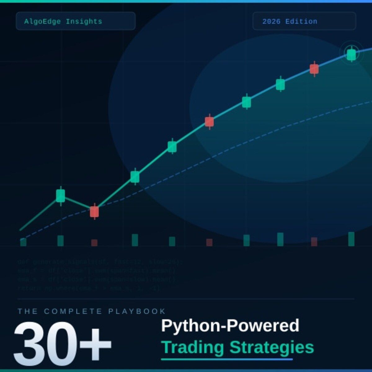
② One strategy in this book returned 2.3× the S&P 500 on a risk-adjusted basis over 5 years.

Fully coded in Python. Yours to run today.

The 2026 Playbook — 30+ backtested strategies,
full code included, ready to deploy.

20% off until Tuesday. Use APRIL2026 at checkout.

$79 → $63.20 · Expires April 7.

→ Grab it before Tuesday

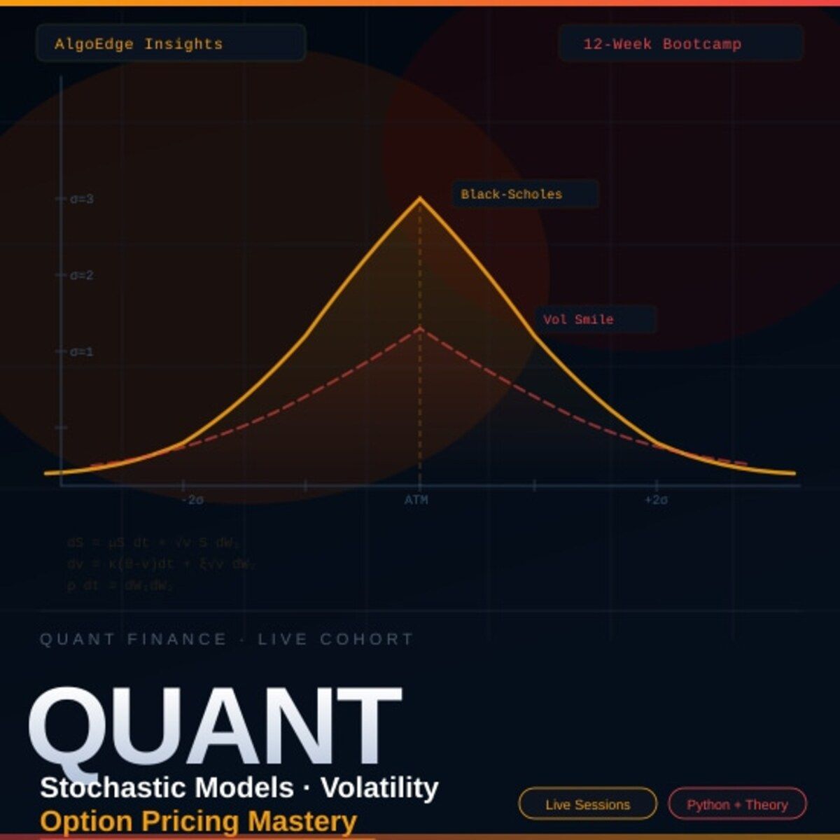
⑤ Most quant courses teach you to watch. This one makes you build.

Live. Weekly. With feedback on your actual code.

The AlgoEdge Quant Finance Bootcamp — 12 weeks of stochastic models, Black-Scholes, Heston, volatility surfaces, and exotic options. Built from scratch in Python.

Not pre-recorded. Not self-paced. Live sessions, weekly homework, direct feedback, and a full code library that's yours to keep.

Cohort size is limited intentionally — so every question gets answered.

→ Before you enroll, reach out for a 15-minute fit check. No pitch, no pressure.

📩 Email first: [email protected]

Premium Members – Your Full Notebook Is Ready

The complete Google Colab notebook from today’s article (with live data, full Hidden Markov Model, interactive charts, statistics, and one-click CSV export) is waiting for you.

Preview of what you’ll get:

Inside the SMA Strategy Lab

  • 📥 Auto-fetches GSPC.INDX data — Integrated with EODHD APIs to pull 10 years of historical daily price action.

  • 📡 Low-Pass Filter Logic — Explains how to separate high-frequency market "noise" from the underlying "signal" using DSP principles.

  • 🛡️ Bias-Free Signal Engine — Implements causal math using .shift(1) to strictly eliminate lookahead bias and "seeing the future."

  • ⚖️ Lag-Length Analysis — Quantifies the trade-off between smoothness and responsiveness ($Lag \approx \frac{N-1}{2}$) across 5 different time horizons.

  • 🔄 Multi-Window Backtester — Runs 10-day, 20-day, 50-day, 100-day, and 200-day Simple Moving Average (SMA) strategies simultaneously.

  • 📊 Risk-Adjusted Scorecard — Calculates Sharpe Ratios, Annualized Volatility, and Max Drawdowns for every window.

  • 📉 Drawdown Heatmaps — Visualizes the peak-to-trough pain for each strategy to identify which window survives market crashes best.

  • 📈 Comparative Visualization — Generates 6+ high-resolution charts, including equity curves, rolling volatility, and performance bar charts.

  • 🗃️ Performance Matrix — Consolidates all results into a clean, rounded pandas table ready for export or further quantitative research.

Free readers – you already got the full breakdown and visuals in the article. Paid members – you get the actual tool.

Not upgraded yet? Fix that in 10 seconds here👇

Google Collab Notebook With Full Code Is Available In the End Of The Article Behind The Paywall 👇 (For Paid Subs Only)

“Without a filter, a man is just chaos walking.” — Patrick Ness 👏

Diagram created by the author using Lucidchart templates.

👋 😀 Hello, market explorers and fellow quants!

Welcome back to the series “Backtesting Ten Basic Moving Averages of S&P 500”!

In Part 1, dedicated to simple averaging techniques, we explored the simple moving average (SMA), focusing on the lag–length dilemma, noise reduction, and the avoidance of lookahead bias [1]. Cumulative MA and Centered MA were deliberately excluded from Part 1 backtesting because of excessive lag and lookahead bias, respectively.

Part 2 further addresses the limitations of the SMA by examining the Weighted Moving Average (WMA) [2].

A WMA is similar to a SMA, but instead of giving equal importance to all observations, it assigns different weights to each data point, usually giving more weight to recent prices [2].

Generally, WMA does a decent job of taming noise. It smooths better than SMA because older prices have less influence, but it can get jumpy if the weights put too much emphasis on recent data. Its lag is moderate and a bit faster than SMA [2].

Let’s take a closer look at these points! 🚀

Contents

· Fetching 10-Year S&P 500 Data
· Multi-Window WMA Backtesting
· WMA vs. SMA: A Risk–Return Analysis
· Takeaways
· Next Steps
· References
· Disclaimer

Go from AI overwhelmed to AI savvy professional

AI will eliminate 300 million jobs in the next 5 years.

Yours doesn't have to be one of them.

Here's how to future-proof your career:

  • Join the Superhuman AI newsletter - read by 1M+ professionals

  • Learn AI skills in 3 mins a day

  • Become the AI expert on your team

Fetching 10-Year S&P 500 Data

Let’s start by collecting 10 years of daily historical price data for GSPC.INDX using the EODHD APIs (cf. Part 1 [1])

import requests
import pandas as pd
import numpy as np
import matplotlib.pyplot as plt
from datetime import datetime, timedelta
# ---------------------------
# CONFIG
# ---------------------------
API_KEY = "YOUR API KEY"

SYMBOL='GSPC.INDX'
# ---------------------------
# DOWNLOAD DATA
# ---------------------------
end_date = datetime.today()
start_date = end_date - timedelta(days=365 * 10)

url = f"https://eodhd.com/api/eod/{SYMBOL}"
params = {
    "from": start_date.strftime("%Y-%m-%d"),
    "to": end_date.strftime("%Y-%m-%d"),
    "period": "d",
    "fmt": "json",
    "api_token": API_KEY
}

data = requests.get(url, params=params).json()
df = pd.DataFrame(data)    # 2513 entries
df['date'] = pd.to_datetime(df['date'])
df.set_index('date', inplace=True)

df.sort_values('date', inplace=True)
df.reset_index(drop=True, inplace=True)  # <- important
prices = df['close']

prices.plot(figsize=(14, 6), title="GSPC.INDX Close Price USD")
plt.ylabel("Price USD")
plt.xlabel("Time Index")
plt.grid()
plt.show()

GSPC.INDX Close Price USD from 2016–03–21 to 2026–03–18 (2513 entries).

This dataset is required to backtest a multi-window, long-only WMA strategy.

Multi-Window WMA Backtesting

Initializations

Calculating the daily returns, which are essential for WMA backtesting

returns = prices.pct_change().fillna(0)

#.fillna(0) replaces that NaN with 0, assuming no gain/loss on the first day.

Defining multiple window lengths to compare performance across short, medium, and long-term WMA

# windows to test
windows = [10, 20, 50, 100, 200]

Initializing empty dictionaries for WMA backtest outputs

results = {} # performance metrics
equity_curves = {} # cumulative returns
drawdowns = {} # drawdowns
volatility = {} # volatility

Implementation

Implementing a complete WMA backtesting loop (step 1)

def WMA(series, window):
    weights = np.arange(1, window + 1)
    return series.rolling(window).apply(
        lambda x: np.dot(x, weights) / weights.sum(),
        raw=True
    )

for w in windows:

    wma = WMA(prices, w)

    signal = (prices > wma).astype(int)
    position = signal.shift(1).fillna(0)

    strat_ret = position * returns
    equity = (1 + strat_ret).cumprod()

    peak = equity.cummax()
    dd = (equity - peak) / peak

    vol = strat_ret.rolling(w).std() * np.sqrt(252)

    equity_curves[w] = equity
    drawdowns[w] = dd
    volatility[w] = vol

    ann_return = equity.iloc[-1] ** (252/len(equity)) - 1
    ann_vol = strat_ret.std() * np.sqrt(252)
    sharpe = ann_return / ann_vol if ann_vol != 0 else 0
    max_dd = dd.min()

    results[w] = {
        "Total Return": equity.iloc[-1] - 1,
        "Annual Return": ann_return,
        "Volatility": ann_vol,
        "Sharpe": sharpe,
        "Max Drawdown": max_dd
    }

perf_wma = pd.DataFrame(results).T

This code correctly simulates real-world trading and avoids lookahead bias:

1. series.rolling(window).apply() only uses the current and past window values to compute the weighted average. It never accesses future prices.

2. position = signal.shift(1).fillna(0) ensures that the trade decision for day t is based on the WMA computed up to day t−1, not the current or future day. This prevents peeking ahead.

3. strat_ret = position * returns multiplies the position (lagged by one day) by the actual return of the next day, which correctly simulates entering the trade at the open of the next day after the signal.

Key Visualizations

Plotting Cumulative Returns of Multi-Window WMA Strategies (step 2)

plt.figure(figsize=(12,6))

for w in windows:
    plt.plot(equity_curves[w], label=f"WMA {w}")

plt.title("Cumulative Returns of Multi-WMA Strategies")
plt.ylabel("Equity")
plt.xlabel("Time")
plt.legend()
plt.grid(True)

plt.show()

Cumulative Returns of Multi-WMA Strategies

Plotting Drawdowns of Multi-Window WMA Strategies (step 3)

plt.figure(figsize=(12,6))

for w in windows:
    plt.plot(drawdowns[w], label=f"WMA {w}")

plt.title("Drawdowns of Multi-WMA Strategies")
plt.ylabel("Drawdown")
plt.xlabel("Time")
plt.legend()
plt.grid(True)

plt.show()

Drawdowns of Multi-WMA Strategies

Plotting Rolling Volatility of Multi-Window WMA Strategies (step 4)

Your Boss Will Think You’re an Ecom Genius

Optimizing for growth? Go-to-Millions is Ari Murray’s ecommerce newsletter packed with proven tactics, creative that converts, and real operator insights—from product strategy to paid media. No mushy strategy. Just what’s working. Subscribe free for weekly ideas that drive revenue.

plt.figure(figsize=(12,6))

for w in windows:
    plt.plot(volatility[w], label=f"WMA {w}")

plt.title("Rolling Volatility of WMA Strategies")
plt.ylabel("Annualized Volatility")
plt.xlabel("Time")
plt.legend()
plt.grid(True)

plt.show()

Rolling Volatility of WMA Strategies

Comparing Multi-Window WMA Total Returns, Sharpe Ratio, and Volatility (step 5)

perf_wma["Total Return"].plot.bar(figsize=(10,5))
plt.title("Total Return Comparison (WMA)")
plt.ylabel("Return")
plt.grid(axis='y')
plt.show()

Total Return Comparison (WMA)

perf_wma["Sharpe"].plot.bar(figsize=(10,5))
plt.title("Sharpe Ratio Comparison (WMA)")
plt.ylabel("Sharpe")
plt.grid(axis='y')
plt.show()

Sharpe Ratio Comparison (WMA)

perf_wma["Volatility"].plot.bar(figsize=(10,5))
plt.title("Volatility Comparison (WMA)")
plt.ylabel("Annualized Volatility")
plt.grid(axis='y')
plt.show()

Volatility Comparison (WMA)

  • Examining the WMA performance table from the backtest (step 6)

print(perf_wma.round(3))

  Total Return  Annual Return  Volatility  Sharpe  Max Drawdown
10          0.700          0.055       0.109   0.504        -0.213
20          0.822          0.062       0.105   0.589        -0.189
50          1.239          0.084       0.104   0.809        -0.196
100         0.858          0.064       0.107   0.601        -0.168
200         1.098          0.077       0.112   0.691        -0.219

Observations:

  • Very short-term WMA is too reactive, producing low returns and moderate risk-adjusted performance. Noise dominates the signals.

  • Medium-term windows perform best, with the 50-day WMA achieving the highest returns and strongest risk-adjusted performance, effectively capturing trends while maintaining reasonable drawdowns.

  • Longer windows smooth out fluctuations. The 100-day window limits drawdowns but delivers moderate returns, while the 200-day window boosts total return at the cost of slightly higher drawdowns, reflecting slower trend responsiveness.

Adding a new column named “MA” and assigning the values “SMA” and “WMA” to all rows for comparison purposes. All rows with the value “SMA” were copied from Part 1 [1]. This allows us to combine backtesting results into a single DataFrame (step 7).

perf_wma['WMA'] = 'WMA'
perf_wma['Window'] = perf_wma.index

perf_combined = pd.DataFrame()
perf_combined = pd.concat([perf_sma, perf_wma])
perf_combined.reset_index(drop=True, inplace=True)
perf_combined['MA'] = perf_combined['MA'].fillna(perf_combined['WMA'])
perf_combined = perf_combined.drop(columns=['WMA'])
print(perf_combined)

  Total Return  Annual Return  Volatility    Sharpe  Max Drawdown   MA  \
0      0.862000       0.064000    0.107000  0.603000     -0.210000  SMA   
1      1.055000       0.075000    0.104000  0.720000     -0.181000  SMA   
2      0.967000       0.070000    0.105000  0.669000     -0.213000  SMA   
3      1.110000       0.078000    0.110000  0.706000     -0.193000  SMA   
4      1.076000       0.076000    0.114000  0.664000     -0.197000  SMA   
5      0.700028       0.054654    0.108528  0.503591     -0.213427  WMA   
6      0.821632       0.061986    0.105294  0.588689     -0.188931  WMA   
7      1.239062       0.084187    0.104018  0.809351     -0.195500  WMA   
8      0.858183       0.064103    0.106682  0.600880     -0.167701  WMA   
9      1.097970       0.077134    0.111633  0.690956     -0.219340  WMA   

   Window  
0      10  
1      20  
2      50  
3     100  
4     200  
5      10  
6      20  
7      50  
8     100  
9     200

Using a Pandas pivot operation to compare multi-window SMA and WMA strategies on a single bar plot (step 8)

pivot_return = perf_combined.pivot(index='Window', columns='MA', values='Total Return')
pivot_sharpe = perf_combined.pivot(index='Window', columns='MA', values='Sharpe')
pivot_vol = perf_combined.pivot(index='Window', columns='MA', values='Volatility')
  • SMA vs WMA Total Return

pivot_return.plot.bar(figsize=(10,6))

plt.title("SMA vs WMA Total Return")
plt.ylabel("Return")
plt.xlabel("Window Length")
plt.grid(axis='y')

plt.show()

SMA vs WMA Total Return

  • SMA vs WMA Sharpe Ratio

pivot_sharpe.plot.bar(figsize=(10,6))

plt.title("SMA vs WMA Sharpe Ratio")
plt.ylabel("Sharpe Ratio")
plt.xlabel("Window Length")
plt.grid(axis='y')

plt.show()

SMA vs WMA Sharpe Ratio

  • SMA vs WMA Volatility

pivot_vol.plot.bar(figsize=(10,6))

plt.title("SMA vs WMA Volatility")
plt.ylabel("Volatility")
plt.xlabel("Window Length")
plt.grid(axis='y')

plt.show()

SMA vs WMA Volatility

WMA vs. SMA: A Risk–Return Analysis

Overall Trend by Window

  • Short windows (10 days): Both SMA (Total Return 0.86, Sharpe 0.60) and WMA (Total Return 0.70, Sharpe 0.50) show weak performance and are noisy. The shorter lookback makes the moving average react too quickly to minor fluctuations, resulting in lower returns and moderate risk-adjusted performance.

  • Medium windows (20–50 days): Performance improves significantly. For SMA at 20 days, the total return reaches 1.055 with Sharpe 0.72, and for WMA at 50 days, the total return jumps to 1.239 with Sharpe 0.81. This indicates that medium-term windows offer the best balance between trend responsiveness and noise reduction.

  • Long windows (100–200 days): SMA shows slightly higher total returns (up to 1.110 at 100 days) but moderate Sharpe ratios (~0.70), while WMA at 200 days shows lower Sharpe (0.69) and returns (1.097). Longer windows provide stability, but may lag market moves, slightly reducing efficiency.

Comparing SMA vs WMA

  • Returns: WMA generally produces higher peak returns, especially at the medium window (50 days: 1.239 vs SMA 50-day 0.967).

  • Sharpe Ratio: WMA also achieves the highest Sharpe overall (0.81) at 50 days, compared to SMA’s peak of 0.72 at 20 days, suggesting better risk-adjusted performance in medium-term windows.

  • Volatility: Both SMA and WMA have similar volatility ranges (~10–11%), so the improved returns from WMA do not come at the cost of excessive risk.

  • Drawdowns: WMA drawdowns vary more by window: lowest at -16.8% (100 days) and slightly higher at -21.9% (200 days), showing that WMA can outperform or underperform depending on the chosen window. SMA drawdowns are more consistent (~-18% to -21%), reflecting its stability

Takeaways

Responsiveness vs Stability Trade-off:

  • SMA is slower but more consistent across windows.

  • WMA is more responsive, capturing trends better in medium-term windows but can be less reliable at extremes.

Optimal Window Selection:

  • For SMA, 20–100 days balances risk and return.

  • For WMA, 50-day window delivers the strongest overall performance.

Risk Management:

  • Both methods keep volatility controlled (~10–11%).

  • Drawdowns remain mostly within acceptable limits (< -22%).

Bottom Line:

Medium-term WMA (50 days) outperforms SMA in both total return and risk-adjusted performance, while SMA remains more stable across different window lengths, and short-term windows for both are too noisy to be effective.

Next Steps

In Parts 3–5, we will compare the performance of WMA against three other popular weighted averaging techniques: EMA, DEMA, and TEMA.

Thank for reading, and see you in the next market adventure! 👋😊

Disclaimer

  • I confirm that they have no financial or personal relationships that could inappropriately influence the content of this article.

  • I declare that no data privacy policy is breached, and that any data associated with the contents here are obtained legitimately to the best of my knowledge.

  • The following disclaimer clarifies that the information provided in this article is for educational use only and should not be considered financial or investment advice.

  • The information provided does not take into account your individual financial situation, objectives, or risk tolerance.

  • Any investment decisions or actions you undertake are solely your responsibility.

  • You should independently evaluate the suitability of any investment based on your financial objectives, risk tolerance, and investment timeframe.

  • It is recommended to seek advice from a certified financial professional who can provide personalized guidance tailored to your specific needs.

  • The tools, data, content, and information offered are impersonal and not customized to meet the investment needs of any individual. As such, the tools, data, content, and information are provided solely for informational and educational purposes only.

  • This article is the author’s original work and has not been published or submitted elsewhere.

  • All images unless otherwise noted are by the author.

logo

Subscribe to our premium content to read the rest.

Become a paying subscriber to get access to this post and other subscriber-only content.

Upgrade

Keep Reading