Does your car insurance cover what really matters?

Not all car insurance is created equal. Minimum liability coverage may keep you legal on the road, but it often won’t be enough to cover the full cost of an accident. Without proper limits, you could be left paying thousands out of pocket. The right policy ensures you and your finances are protected. Check out Money’s car insurance tool to get the coverage you actually need.
Elite Quant Plan – 14-Day Free Trial (This Week Only)
No card needed. Cancel anytime. Zero risk.
You get immediate access to:
Full code from every article (including today’s HMM notebook)
Private GitHub repos & templates
All premium deep dives (3–5 per month)
2 × 1-on-1 calls with me
One custom bot built/fixed for you
Try the entire Elite experience for 14 days — completely free.
→ Start your free trial now 👇
(Doors close in 7 days or when the post goes out of the spotlight — whichever comes first.)
See you on the inside.
👉 Upgrade Now →
🔔 Limited-Time Holiday Deal: 20% Off Our Complete 2026 Playbook! 🔔
Level up before the year ends!
AlgoEdge Insights: 30+ Python-Powered Trading Strategies – The Complete 2026 Playbook
30+ battle-tested algorithmic trading strategies from the AlgoEdge Insights newsletter – fully coded in Python, backtested, and ready to deploy. Your full arsenal for dominating 2026 markets.
Special Promo: Use code DECEMBER2025 for 20% off
Valid only until December 20, 2025 — act fast!
👇 Buy Now & Save 👇
Instant access to every strategy we've shared, plus exclusive extras.
— AlgoEdge Insights Team
Premium Members – Your Full Notebook Is Ready
The complete Google Colab notebook from today’s article (with live data, full Hidden Markov Model, interactive charts, statistics, and one-click CSV export) is waiting for you.
Preview of what you’ll get:

Inside:
Automatic gold data from 2008 to today (GC=F via yfinance)
Real 3-state Gaussian model using GaussianMixture from scikit-learn – clusters daily returns + volatility into Low/Medium/High regimes (robust & realistic alternative to HMM)
Smart regime labeling by sorting on average volatility
Beautiful interactive Plotly charts (zoom, hover, dark mode):
Price with colored regime shading
Volatility over time with regimes
Cumulative returns broken down by regime
Detailed performance table (days, % time, returns, volatility)
Ready-to-use CSV export with all data + regime labels
One-line switch for Bitcoin, S&P 500, or any ticker
Free readers – you already got the full breakdown and visuals in the article. Paid members – you get the actual tool.
Not upgraded yet? Fix that in 10 seconds here👇
Google Collab Notebook With Full Code Is Available In the End Of The Article Behind The Paywall 👇 (For Paid Subs Only)

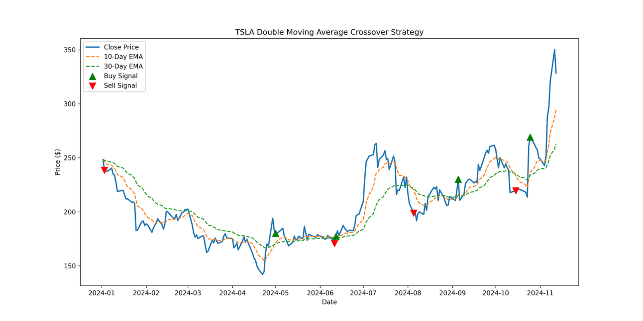
Tesla Double Moving Average Crossover Strategy Chart
Introduction
The Double Moving Average Crossover is one of the simplest yet powerful trading strategies used by both beginners and seasoned traders. By using two different moving averages, this strategy identifies potential buy and sell signals when the faster moving average crosses over or under a slower one. In this article, we’ll dive into the details of how to implement this strategy in Python, backtest it, and analyze the results.
Last Time the Market Was This Expensive, Investors Waited 14 Years to Break Even
In 1999, the S&P 500 peaked. Then it took 14 years to gradually recover by 2013.
Today? Goldman Sachs sounds crazy forecasting 3% returns for 2024 to 2034.
But we’re currently seeing the highest price for the S&P 500 compared to earnings since the dot-com boom.
So, maybe that’s why they’re not alone; Vanguard projects about 5%.
In fact, now just about everything seems priced near all time highs. Equities, gold, crypto, etc.
But billionaires have long diversified a slice of their portfolios with one asset class that is poised to rebound.
It’s post war and contemporary art.
Sounds crazy, but over 70,000 investors have followed suit since 2019—with Masterworks.
You can invest in shares of artworks featuring Banksy, Basquiat, Picasso, and more.
24 exits later, results speak for themselves: net annualized returns like 14.6%, 17.6%, and 17.8%.*
My subscribers can skip the waitlist.
*Investing involves risk. Past performance is not indicative of future returns. Important Reg A disclosures: masterworks.com/cd.
What is a Double Moving Average Crossover?
The Double Moving Average Crossover strategy relies on two exponential moving averages (EMAs):
Short-term Moving Average (fast): This moving average responds quickly to recent price changes.
Long-term Moving Average (slow): This one reacts more slowly to price changes, capturing long-term trends.
Key Signals:
Buy Signal: When the short-term EMA crosses above the long-term EMA, indicating an upward trend.
Sell Signal: When the short-term EMA crosses below the long-term EMA, indicating a downward trend.
This strategy works well in trending markets but may generate false signals during sideways (range-bound) markets.
Advantages
Simplicity: The strategy’s logic is straightforward and easy to understand, making it accessible for traders with varying levels of experience.
Trend-Following: By identifying crossovers, the strategy aligns with prevailing trends, making it effective in trending markets where it can capture substantial price movements.
Reduced Emotional Bias: Using systematic moving average rules helps traders reduce emotional bias, leading to more consistent decision-making.
Customizable: Moving averages can be adjusted based on time frames and trading goals, allowing for flexibility across different asset classes and market conditions.
Disadvantages
Lagging Indicators: Moving averages are inherently lagging, so this strategy often signals a buy or sell after the trend has begun. This lag can result in delayed entry or exit.
False Signals in Range-Bound Markets: In sideways or range-bound markets, the crossover signals can be frequent and misleading, leading to “whipsaw” trades and potential losses.
Limited Predictive Power: Since moving averages are calculated based on historical prices, they do not predict future prices but rather follow the trend, which may be unsuitable for highly volatile markets.
Important Considerations
Time Frame Selection: The moving average lengths you choose greatly affect the strategy’s performance. Shorter moving averages provide more frequent signals but increase the chance of false signals, while longer moving averages are more stable but may miss shorter trends.
Market Conditions: This strategy is most effective in trending markets. In range-bound conditions, additional filters (like using volume or other indicators) may help to avoid false signals.
Risk Management: As with any trading strategy, risk management techniques like setting stop losses and using position sizing are essential to protect capital.
Backtesting and Optimization: Regularly backtesting and fine-tuning this strategy with historical data helps to understand how it performs under different market conditions, making it more reliable for real-world trading.
Simulate the Strategy in Python
We now simulate the Double Moving Average Crossover Strategy on historical data.
Setting Up the Environment
To implement this strategy, you’ll need Python along with a few essential libraries. In your python environment, install the following libraries:
pip install pandas numpy matplotlib yfinanceImporting Libraries
Import the libraries in a .ipynb notebook:
import pandas as pd
import numpy as np
import matplotlib.pyplot as plt
import yfinance as yf
from tabulate import tabulate
from datetime import datetime
Data
We’ll use historical data from Yahoo Finance to apply our strategy. For this example, let’s use Tesla’s stock (TSLA).
# Define the stock symbol and the date range for our data
stock_symbol = 'TSLA'
start_date = '2024-01-01'
end_date = datetime.today().strftime('%Y-%m-%d')  # Sets end date to today's date
print(f"Double Moving Average Crossover Trading for: {stock_symbol}\nStart Date: {start_date}\nEnd Date: {end_date}")
After downloading the data, we can now preprocess it for easy strategy simulation:
df = yf.download(stock_symbol, start=start_date, end=end_date)

# Select the desired columns (first level of MultiIndex)
df.columns = df.columns.get_level_values(0)

# Keep only the columns you are interested in
df = df[['Open', 'Close', 'Volume', 'Low', 'High']]

# If the index already contains the dates, rename the index
df.index.name = 'Date'  # Ensure the index is named "Date"

# Resetting the index if necessary
df.reset_index(inplace=True)

# Ensure that the index is of type datetime
df['Date'] = pd.to_datetime(df['Date'])

# Set the 'Date' column as the index again (in case it's reset)
df.set_index('Date', inplace=True)

df.head()
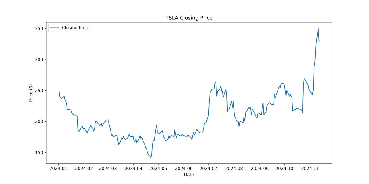
Visualize the Chart
# Plot the closing price
plt.figure(figsize=(12, 6))

plt.plot(df['Close'], label='Closing Price')

# Add title, labels, and legend
plt.title(f'{stock_symbol} Closing Price')
plt.xlabel('Date')
plt.ylabel('Price ($)')
plt.legend()

# Save the plot in 300dpi
plt.savefig(f'{stock_symbol}_stock_chart.png', dpi=300)

# Show the plot
plt.show()
Tesla Stock Price Chart
Calculating Moving Averages
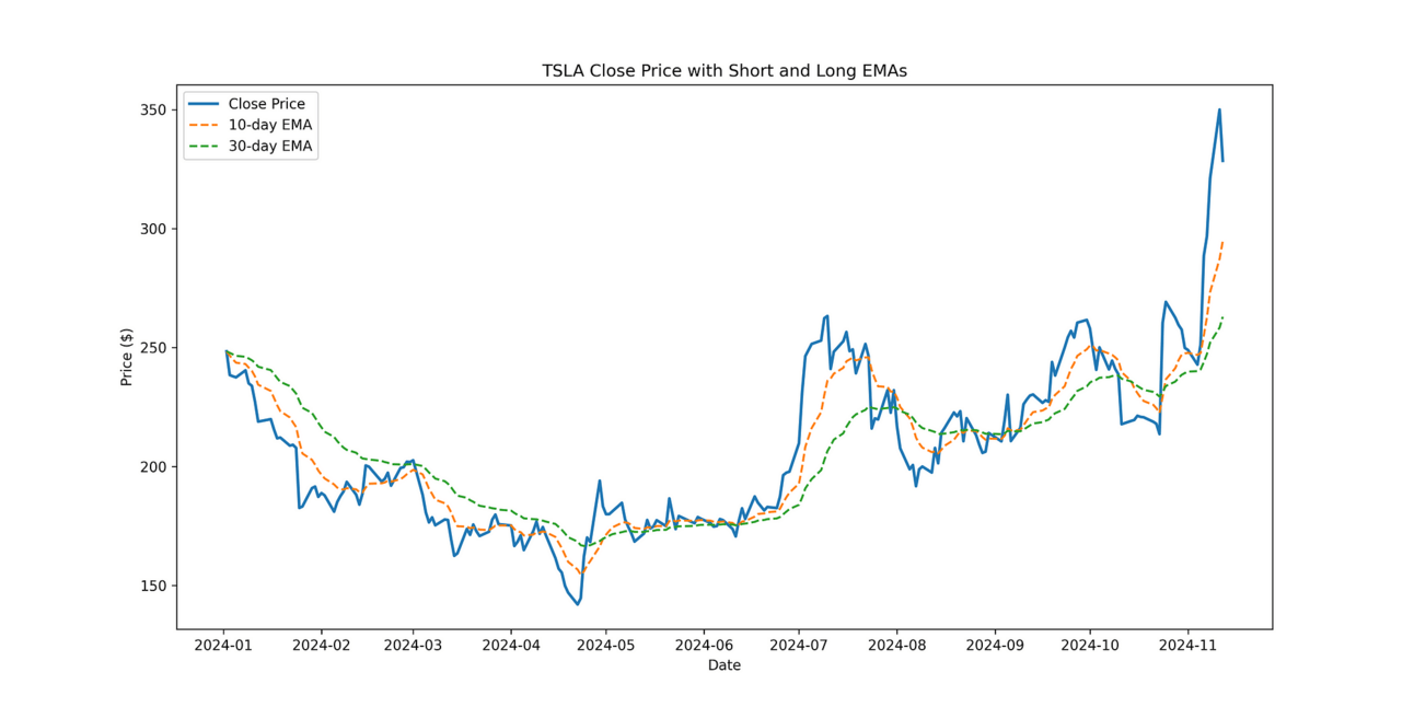
In this section, we calculate the short-term and long-term Exponential Moving Averages (EMAs) using two window sizes, a long and short window. The short-term EMA reacts faster to recent price changes, while the long-term EMA smooths out fluctuations to highlight longer-term trends. These moving averages help in identifying crossover points for potential buy and sell signals.
# Calculate the short and long EMAs
SHORT_WINDOW = 10
LONG_WINDOW = 30
df['SHORT_WINDOW'] = df['Close'].ewm(span=SHORT_WINDOW, adjust=False).mean()
df['LONG_WINDOW'] = df['Close'].ewm(span=LONG_WINDOW, adjust=False).mean()
Visualize the Moving Averages
# Plot the Close Price and EMAs
plt.figure(figsize=(14, 7))

# Plot Close Price
plt.plot(df.index, df['Close'], label='Close Price', linewidth=2)

# Plot Short-term EMA
plt.plot(df.index, df['SHORT_WINDOW'], label=f'{SHORT_WINDOW}-day EMA', linestyle='--')

# Plot Long-term EMA
plt.plot(df.index, df['LONG_WINDOW'], label=f'{LONG_WINDOW}-day EMA', linestyle='--')

# Labels and title
plt.xlabel('Date')
plt.ylabel('Price ($)')
plt.title(f'{stock_symbol} Close Price with Short and Long EMAs')
plt.legend()

# Save plot in 300dpi
plt.savefig(f'{stock_symbol}_moving_averages.png', dpi=300)

plt.show()
Tesla Stock Chart with Moving Averages
Creating Buy and Sell Signals
We’ll add a Signal column to store buy and sell signals based on crossover points.
# Generate buy and sell signals in a single column
df['Signal'] = np.where(
    (df['SHORT_WINDOW'] > df['LONG_WINDOW']) & (df['SHORT_WINDOW'].shift(1) <= df['LONG_WINDOW'].shift(1)), 1,  # Buy Signal
    np.where(
        (df['SHORT_WINDOW'] < df['LONG_WINDOW']) & (df['SHORT_WINDOW'].shift(1) >= df['LONG_WINDOW'].shift(1)), -1,  # Sell Signal
        0  # No Signal
    )
)
Simulate the Strategy
Calculate the Brokerage Fee
We define a function to calculate the brokerage fee for each transaction. The fee is set to 0.25% of the transaction amount, with a minimum fee of $0.01 to ensure that small transactions still incur a reasonable fee. This helps simulate the costs associated with trading, making the strategy more realistic.
# Define the fee calculation function
def calculate_fee(amount: float) -> float:
    """Calculate the brokerage fee based on transaction amount."""
    fee = amount * 0.0025  # 0.25% of the transaction
    return max(fee, 0.01)   # Minimum fee of $0.01
Run Backtest
# Starting capital
initial_cash = 100  # Example initial capital
cash = initial_cash
shares = 0
df['Portfolio Value'] = cash

# List to store transaction details for tabulation
transaction_details = []

for i, row in df.iterrows():
    if row['Signal'] == 1 and cash > 0:  # Buy condition
        # Calculate the fee for the buy transaction
        fee = calculate_fee(cash)

        # Calculate how many shares can be bought after deducting the fee
        shares_bought = (cash - fee) / row['Close']

        # Deduct the cash and fee for the purchase
        cash -= shares_bought * row['Close'] + fee

        # Add the bought shares to the portfolio
        shares += shares_bought

        # Record transaction details
        transaction_details.append([row.name, 'Buy', round(row['Close'], 2), round(fee, 2), round(cash + (shares * row['Close']), 2)])

    elif row['Signal'] == -1 and shares > 0:  # Sell condition
        # Calculate how much cash is earned from selling shares
        total_sale_amount = shares * row['Close']

        # Calculate the fee for the sell transaction
        fee = calculate_fee(total_sale_amount)

        # Cash earned after the fee is deducted
        cash_earned = total_sale_amount - fee

        # Update the cash balance after selling shares
        cash += cash_earned

        # All shares are sold
        shares = 0

        # Record transaction details
        transaction_details.append([row.name, 'Sell', round(row['Close'], 2), round(fee, 2), round(cash, 2)])

    # Update portfolio value
    df.at[i, 'Portfolio Value'] = cash + (shares * row['Close'])

# Summarize results using tabulate
print(tabulate(transaction_details, headers=["Date", "Action", "Price ($)", "Fee ($)", "Portfolio Value ($)"], tablefmt="pretty"))

# Final performance
final_value = cash + (shares * df.iloc[-1]['Close'])
profit = final_value - initial_cash
print(f"\nFinal Portfolio Value: ${final_value:.2f}")
print(f"Total Profit/Loss: ${profit:.2f}")
Analyzing the Results
Tabulate Buys and Sells
The code above shows a table similar to the one below where they buys and sells are shown alongside their fees and the portfolio value. We can see that this strategy with a SHORT_WINDOW = 10 and LONG_WINDOW = 30 leads to a profit of $21.67 from 01 January 2024 to 13 November 2024 .
+---------------------------+--------+-----------+---------+---------------------+
|           Date            | Action | Price ($) | Fee ($) | Portfolio Value ($) |
+---------------------------+--------+-----------+---------+---------------------+
| 2024-05-01 00:00:00+00:00 |  Buy   |  179.99   |  0.25   |        99.75        |
| 2024-06-11 00:00:00+00:00 |  Sell  |  170.66   |  0.24   |        94.34        |
| 2024-06-12 00:00:00+00:00 |  Buy   |  177.29   |  0.24   |        94.11        |
| 2024-08-05 00:00:00+00:00 |  Sell  |  198.88   |  0.26   |        105.3        |
| 2024-09-05 00:00:00+00:00 |  Buy   |  230.17   |  0.26   |       105.04        |
| 2024-10-15 00:00:00+00:00 |  Sell  |  219.57   |  0.25   |        99.95        |
| 2024-10-25 00:00:00+00:00 |  Buy   |  269.19   |  0.25   |        99.7         |
+---------------------------+--------+-----------+---------+---------------------+

Initial Portfolio Vaue: $100.00
Final Portfolio Value: $121.67
Total Profit/Loss: $21.67
Visualize the Buys and Sells
We can now visualize when the buys and sells are made. From this we can adjust our window sizes accordingly.

Tesla Stock Price, Moving Averages and Buy/Sell Signals
Conclusion
The Double Moving Average Crossover Strategy is a straightforward yet effective approach to trading in trending markets. However, remember that no strategy is foolproof. Backtesting on various stocks and timeframes can help you understand how it performs under different market conditions. Implementing a trailing stop or combining this strategy with other indicators like the RSI can further improve its robustness.
Subscribe to our premium content to read the rest.
Become a paying subscriber to get access to this post and other subscriber-only content.
Upgrade


