
In partnership with

Invest right from your couch

Have you always been kind of interested in investing but found it too intimidating (or just plain boring)? Yeah, we get it. Luckily, today’s brokers are a little less Wall Street and much more accessible. Online stockbrokers provide a much more user-friendly experience to buy and sell stocks—right from your couch. Money.com put together a list of the Best Online Stock Brokers to help you open your first account. Check it out!
Elite Quant Plan – 14-Day Free Trial (This Week Only)
No card needed. Cancel anytime. Zero risk.
You get immediate access to:
Full code from every article (including today’s HMM notebook)
Private GitHub repos & templates
All premium deep dives (3–5 per month)
2 × 1-on-1 calls with me
One custom bot built/fixed for you
Try the entire Elite experience for 14 days — completely free.
→ Start your free trial now 👇
(Doors close in 7 days or when the post goes out of the spotlight — whichever comes first.)
See you on the inside.
👉 Upgrade Now →
🔔 Limited-Time Holiday Deal: 20% Off Our Complete 2026 Playbook! 🔔
Level up before the year ends!
AlgoEdge Insights: 30+ Python-Powered Trading Strategies – The Complete 2026 Playbook
30+ battle-tested algorithmic trading strategies from the AlgoEdge Insights newsletter – fully coded in Python, backtested, and ready to deploy. Your full arsenal for dominating 2026 markets.
Special Promo: Use code DECEMBER2025 for 20% off
Valid only until December 20, 2025 — act fast!
👇 Buy Now & Save 👇

Instant access to every strategy we've shared, plus exclusive extras.
— AlgoEdge Insights Team
Premium Members – Your Full Notebook Is Ready
The complete Google Colab notebook from today’s article (with live data, full Hidden Markov Model, interactive charts, statistics, and one-click CSV export) is waiting for you.
Preview of what you’ll get:

Inside:
Downloads historical daily Bitcoin (BTC-USD) price data from Yahoo Finance, starting from September 2014 up to the current date (around 2025).
Cleans the data by adjusting column names to standard OHLCV (Open, High, Low, Close, Volume).
There is a section for plotting the closing price chart (though the provided snippet shows a confusion matrix plot instead, suggesting the notebook includes visualization of results).
The notebook sets up technical indicators using the 'ta' library (though not fully shown in the snippet).
Prepares features and a target label (likely future price direction: 1 for up, 0 for down).
Splits data into training and testing sets.
Trains a Random Forest Classifier on the features.
Free readers – you already got the full breakdown and visuals in the article. Paid members – you get the actual tool.
Not upgraded yet? Fix that in 10 seconds here👇
Google Collab Notebook With Full Code Is Available In the End Of The Article Behind The Paywall 👇 (For Paid Subs Only)

Bitcoin’s Predicted Market Direction
Bitcoin’s price is known for its volatility, offering a valuable dataset for applying machine learning techniques to financial forecasting.
In this project, we focus on predicting whether Bitcoin’s price will move up or down the next day. We use historical price data and engineered technical indicators as input features.
This article covers the full process: data collection, preprocessing, feature engineering, feature selection, model training with a Random Forest classifier, and evaluating the model’s performance.
But what can you actually DO about the proclaimed ‘AI bubble’? Billionaires know an alternative…

Sure, if you held your stocks since the dotcom bubble, you would’ve been up—eventually. But three years after the dot-com bust the S&P 500 was still far down from its peak. So, how else can you invest when almost every market is tied to stocks?
Lo and behold, billionaires have an alternative way to diversify: allocate to a physical asset class that outpaced the S&P by 15% from 1995 to 2025, with almost no correlation to equities. It’s part of a massive global market, long leveraged by the ultra-wealthy (Bezos, Gates, Rockefellers etc).
Contemporary and post-war art.
Masterworks lets you invest in multimillion-dollar artworks featuring legends like Banksy, Basquiat, and Picasso—without needing millions. Over 70,000 members have together invested more than $1.2 billion across over 500 artworks. So far, 25 sales have delivered net annualized returns like 14.6%, 17.6%, and 17.8%.*
Want access?
Investing involves risk. Past performance not indicative of future returns. Reg A disclosures at masterworks.com/cd
Installing Required Libraries
We begin by installing the Python packages used in this notebook. Each of these plays a critical role:
yfinance:to retrieve historical Bitcoin price data from Yahoo Finance.matplotlibandseaborn:for visualizing data and model performance.scikit-learn:to build, train, and evaluate the machine learning model.ta:to compute technical indicators like RSI and MACD.
%pip install yfinance matplotlib scikit-learn seaborn taImporting Libraries and Setting Plot Style
We then import all the relevant packages.
import yfinance as yf
import matplotlib.pyplot as plt
import seaborn as sns
from sklearn.ensemble import RandomForestClassifier
from sklearn.model_selection import train_test_split
from sklearn.metrics import classification_report, confusion_matrix
from sklearn.feature_selection import SelectKBest, f_classif
import ta
Downloading Historical Bitcoin Data
We use yfinance to download historical Bitcoin data from Yahoo Finance.
This dataset includes columns like Open, High, Low, Close, and Volume from Bitcoin’s inception in 2010 up to May 2025.
BTC-USDis the ticker for Bitcoin in US dollars.
data = yf.download("BTC-USD", start="2010-09-17", end="2025-05-19", auto_adjust=True)
data.head()
Selecting and Simplifying Columns
Some data providers like Yahoo Finance return multi-indexed columns. To make our dataset easier to work with, we:
Flatten the columns by selecting the top level.
Keep only the essential fields for price prediction:
Open,Close,Volume,Low, andHigh.
data.columns = data.columns.get_level_values(0)
data = data[['Open', 'Close', 'Volume', 'Low', 'High']]
Visualizing the Close Price
We display the historical closing price of Bitcoin.
plt.figure(figsize=(14, 6))
plt.plot(data.index, data['Close'], label='Close', color='blue')
plt.title('Close Price Over Time')
plt.xlabel('Date')
plt.ylabel('Close Price (USD)')
plt.legend()
plt.grid(True)
plt.savefig("Close.png")
plt.show()
Bitcoin’s Closing Price Over Time
Creating the Target Variable
Our goal is to predict the direction of Bitcoin’s price the next day. So we create a binary target:
1if tomorrow's close is higher than today’s (price went up).0if it’s not (price went down or stayed the same).
We also drop rows with missing values caused by shifting.
data["Direction"] = (data["Close"].shift(-1) > data["Close"]).astype(int)
data.dropna(inplace=True)
Feature Engineering
To improve the predictive power of our model, we create new features derived from the raw price and volume data.
These engineered features help capture important market behaviors such as momentum, volatility, and trend strength that are not immediately obvious from the original data.
Return-Based Features
These features capture how much the price has changed over different time horizons. They help the model understand recent momentum and volatility:
Return_1d— daily return.Return_3d— 3-day return.Return_7d— 7-day return.
data["Return_1d"] = data["Close"].pct_change()
data["Return_3d"] = data["Close"].pct_change(3)
data["Return_7d"] = data["Close"].pct_change(7)
Price Range and Volatility Indicators
We compute features that quantify the price range and price volatility:
High_Low— difference between the daily high and low.Close_Open— intraday price movement.Volatility_7d— rolling 7-day standard deviation of closing prices.
data["High_Low"] = data["High"] - data["Low"]
data["Close_Open"] = data["Close"] - data["Open"]
data["Volatility_7d"] = data["Close"].rolling(7).std()
Moving Averages and Ratios
Moving averages smooth out short-term fluctuations and highlight trends.
We also compute the ratio between two moving averages to capture crossover patterns:
MA_5andMA_10— 5-day and 10-day moving averages.MA_ratio— relative trend strength over short and medium term.
data["MA_5"] = data["Close"].rolling(window=5).mean()
data["MA_10"] = data["Close"].rolling(window=10).mean()
data["MA_ratio"] = data["MA_5"] / data["MA_10"]
RSI Indicator
We use the ta library to calculate the Relative Strength Index (RSI), a momentum indicator that measures overbought or oversold conditions.
data["RSI"] = ta.momentum.RSIIndicator(data["Close"]).rsi()MACD Indicator
We calculate the MACD (Moving Average Convergence Divergence) and its signal line.
These are commonly used in trading strategies to detect shifts in momentum.
macd = ta.trend.MACD(data["Close"])
data["MACD"] = macd.macd()
data["MACD_signal"] = macd.macd_signal()
Volume-Based Features
Volume can confirm price movements. We compute:
Volume_Change— daily percentage change in volume.Volume_MA_5— 5-day moving average of volume.
data["Volume_Change"] = data["Volume"].pct_change()
data["Volume_MA_5"] = data["Volume"].rolling(5).mean()
Lag Features
Lagged features provide the model with recent values of price and volume:
Close_lag_1,Close_lag_2, etc. — yesterday’s and earlier close prices.Volume_lag_1, etc. — volume from previous days.
for lag in range(1, 4):
    data[f"Close_lag_{lag}"] = data["Close"].shift(lag)
    data[f"Volume_lag_{lag}"] = data["Volume"].shift(lag)
Calendar Features
We extract the day of the week and the month to help capture patterns like weekday effects or seasonal trends.
data["DayOfWeek"] = data.index.dayofweek  # Monday=0, Sunday=6
data["Month"] = data.index.month
Momentum and Rolling Extremes
These features help detect the strength and boundaries of trends:
Momentum_10— price change over the past 10 days.Rolling_Max_10,Rolling_Min_10— recent highest and lowest close prices.
data["Momentum_10"] = data["Close"] - data["Close"].shift(10)
data["Rolling_Max_10"] = data["Close"].rolling(10).max()
data["Rolling_Min_10"] = data["Close"].rolling(10).min()
Dropping Missing Values
All the above transformations may introduce NaN values. We remove these rows to clean the dataset.
data.dropna(inplace=True)Preparing the Feature Matrix and Target
We separate our dataset into:
X: feature matrix (all columns except the target).y: target variable indicating if the price went up (1) or not (0).
X = data.drop(columns=["Direction"])
y = data["Direction"]
Feature Selection with SelectKBest
We use SelectKBest with the ANOVA F-test to select the 10 most informative features.
This helps reduce noise and improve model performance.
selector = SelectKBest(score_func=f_classif, k=10)
X_selected = selector.fit_transform(X, y)
Visualizing Feature Importance
We plot the F-scores of the top 10 selected features to understand which ones contributed most to the target.
# Get scores and mask of selected features
scores = selector.scores_
selected_mask = selector.get_support()  # boolean mask of selected features
selected_feature_names = X.columns[selected_mask]

# Plot
plt.figure(figsize=(14, 6))
plt.barh(selected_feature_names, scores[selected_mask], color="teal")
plt.xlabel("F-score")
plt.title("Top 5 Selected Features by F-score (SelectKBest)")
plt.gca().invert_yaxis()  # optional: put highest on top
plt.tight_layout()
plt.savefig("feature_importance.png")
plt.show()
Feature Importance from SelectKBest Feature Selection
Splitting the Data
We split the dataset into training and testing sets using an 80/20 ratio. Note: shuffle=False is used to preserve the time-series order.
X_train, X_test, y_train, y_test = train_test_split(
    X_selected, y, test_size=0.2, random_state=42, shuffle=False
)
Training the Random Forest Model
We train a RandomForestClassifier to learn the relationship between features and the target.
class_weight='balanced'ensures that the model accounts for class imbalance if any.
model = RandomForestClassifier(n_estimators=100, random_state=42, class_weight='balanced')
model.fit(X_train, y_train)
Generating Predictions and Evaluating Performance
We make predictions on the test set and print a classification report including precision, recall, and F1-score.
y_pred = model.predict(X_test)
print(classification_report(y_test, y_pred))
precision recall f1-score support
0 0.51 0.78 0.62 380
1 0.57 0.28 0.38 393
accuracy 0.53 773
macro avg 0.54 0.53 0.50 773
weighted avg 0.54 0.53 0.50 773Visualizing Predictions vs Market Movements
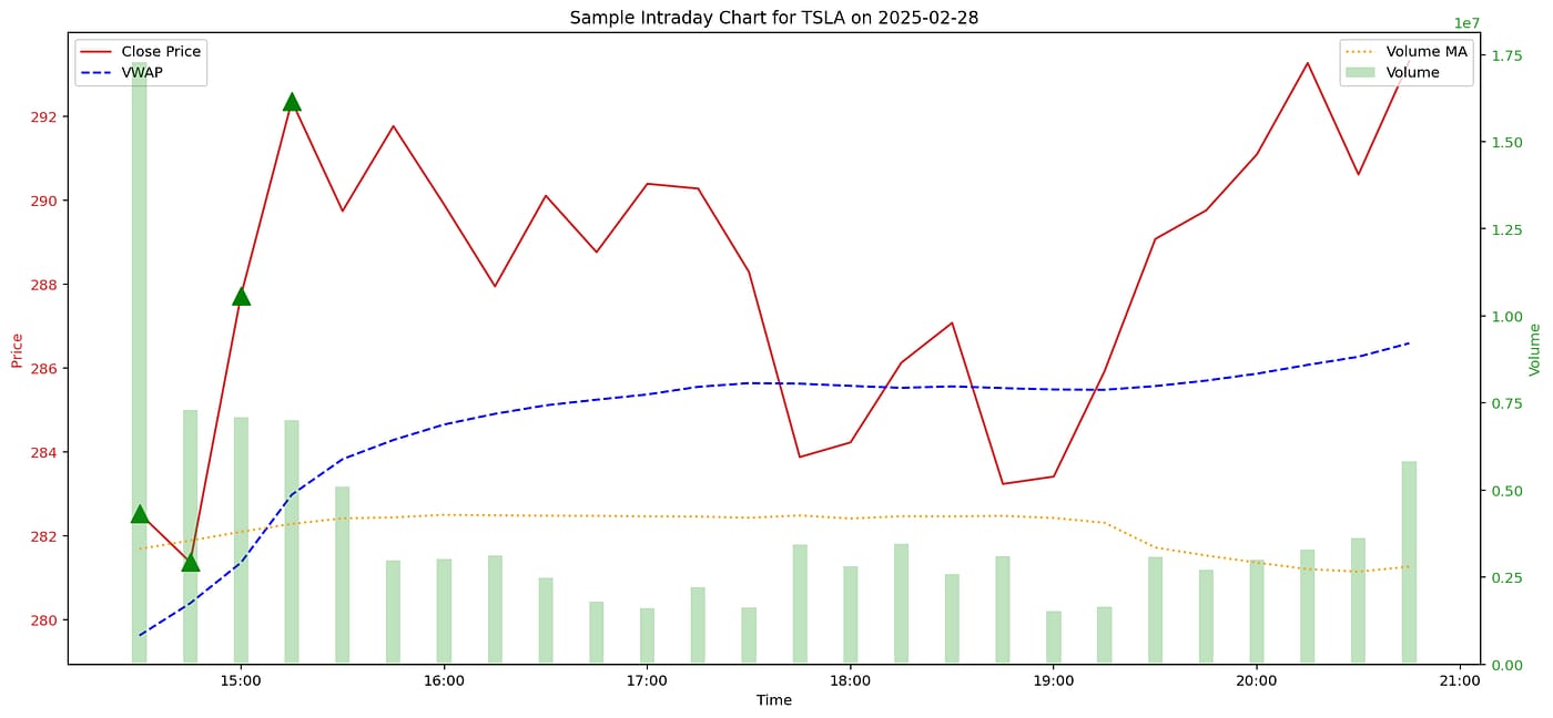
This plot overlays model predictions on Bitcoin’s closing price:
Green triangles indicate days where the model predicted an upward movement.
Red triangles indicate predicted downward movements.
plt.figure(figsize=(14,6))
plt.plot(data.index[-len(y_test):], data["Close"][-len(y_test):], label='Close Price')
plt.plot(data.index[-len(y_test):][y_pred == 1], data["Close"][-len(y_test):][y_pred == 1], '^', markersize=10, color='g', label='Predicted Up')
plt.plot(data.index[-len(y_test):][y_pred == 0], data["Close"][-len(y_test):][y_pred == 0], 'v', markersize=10, color='r', label='Predicted Down')
plt.title("Predicted Bitcoin Direction vs Close Price")
plt.legend()
plt.savefig("predicted_market_direction.png")
plt.show()
Predicted Bitcoin Direction vs Close Price
Confusion Matrix
A confusion matrix gives a snapshot of how many predictions were correct and incorrect. It distinguishes:
True positives (correctly predicted ups).
True negatives (correctly predicted downs).
False positives and false negatives.
cm = confusion_matrix(y_test, y_pred)
sns.heatmap(cm, annot=True, fmt='d', cmap='Blues')
plt.xlabel('Predicted')
plt.ylabel('Actual')
plt.title('Confusion Matrix')
plt.savefig("confusion_matrix.png")
plt.show()
Confusion Matrix
This project demonstrates how machine learning and thoughtful feature engineering can be used to predict the direction of Bitcoin’s price.
While our model makes use of simple technical indicators and historical data, real-world trading strategies would require additional considerations such as transaction costs, slippage, and risk management.
Subscribe to our premium content to read the rest.
Become a paying subscriber to get access to this post and other subscriber-only content.
Upgrade