
In partnership with

The Volatility Cone: A Quant's Tool for Mapping Price Uncertainty
88% resolved. 22% stayed loyal. What went wrong?

That's the AI paradox hiding in your CX stack. Tickets close. Customers leave. And most teams don't see it coming because they're measuring the wrong things.
Efficiency metrics look great on paper. Handle time down. Containment rate up. But customer loyalty? That's a different story — and it's one your current dashboards probably aren't telling you.
Gladly's 2026 Customer Expectations Report surveyed thousands of real consumers to find out exactly where AI-powered service breaks trust, and what separates the platforms that drive retention from the ones that quietly erode it.
If you're architecting the CX stack, this is the data you need to build it right. Not just fast. Not just cheap. Built to last.
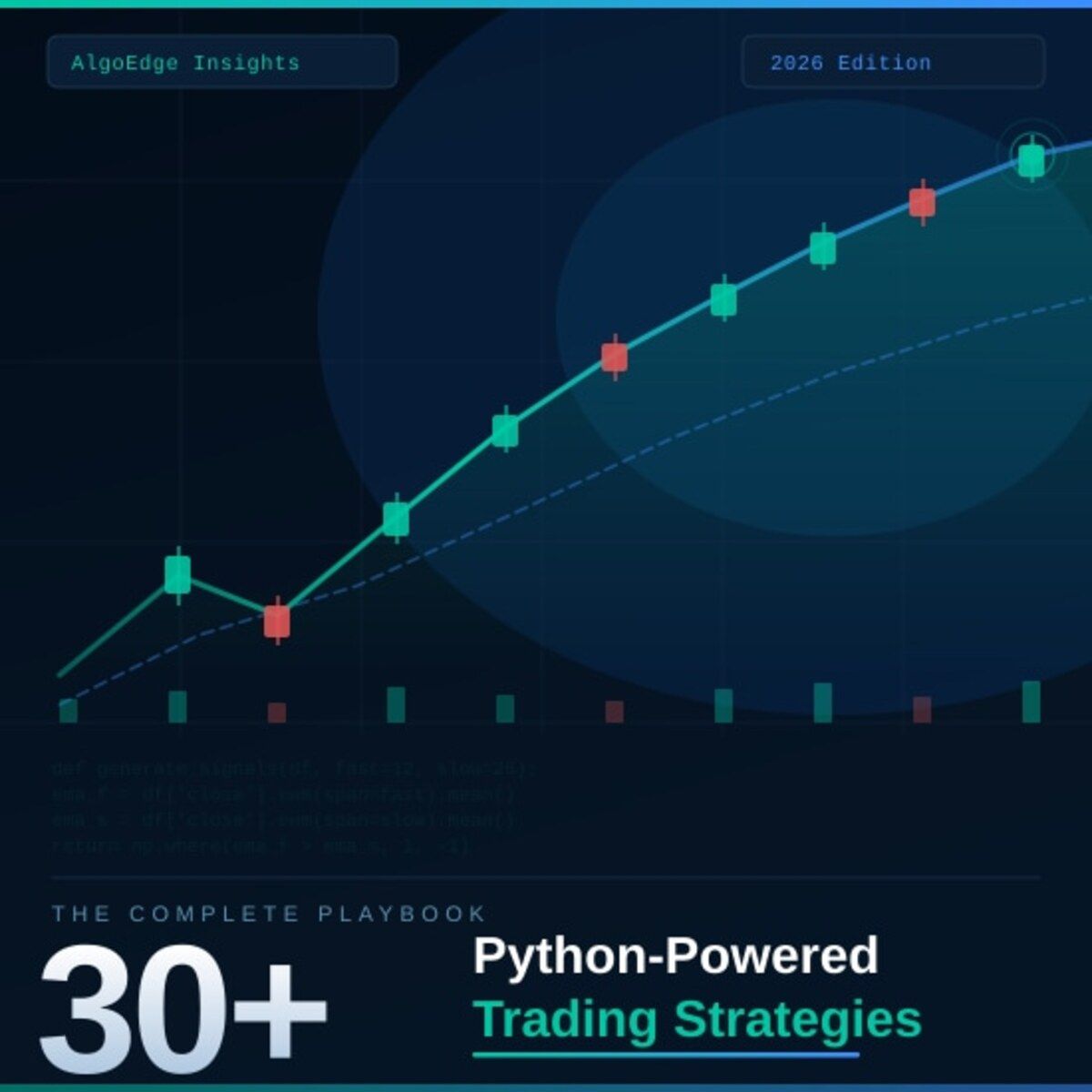
② One strategy in this book returned 2.3× the S&P 500 on a risk-adjusted basis over 5 years.
Fully coded in Python. Yours to run today.
The 2026 Playbook — 30+ backtested strategies,
full code included, ready to deploy.
20% off until Tuesday. Use SPRING2026 at checkout.
$79 → $63.20 · Expires March 31.
→ Grab it before Tuesday
⑤ Most quant courses teach you to watch. This one makes you build.
Live. Weekly. With feedback on your actual code.
The AlgoEdge Quant Finance Bootcamp — 12 weeks of stochastic models, Black-Scholes, Heston, volatility surfaces, and exotic options. Built from scratch in Python.
Not pre-recorded. Not self-paced. Live sessions, weekly homework, direct feedback, and a full code library that's yours to keep.
Cohort size is limited intentionally — so every question gets answered.
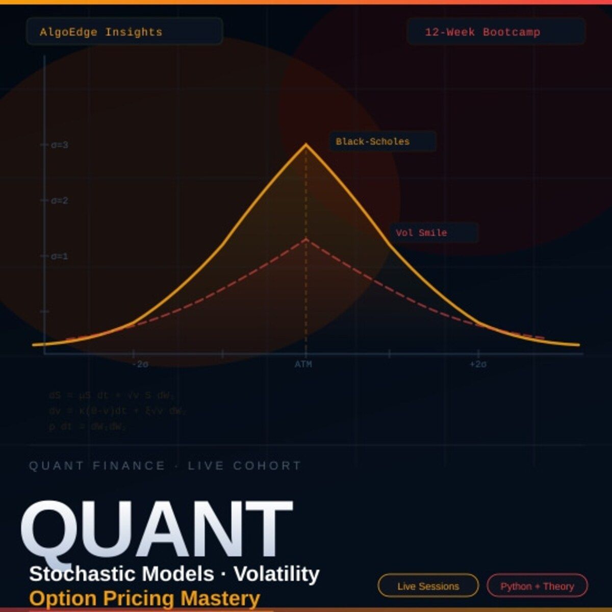
→ Before you enroll, reach out for a 15-minute fit check. No pitch, no pressure.
📩 Email first: [email protected]
Premium Members – Your Full Notebook Is Ready
The complete Google Colab notebook from today’s article (with live data, full Hidden Markov Model, interactive charts, statistics, and one-click CSV export) is waiting for you.
Preview of what you’ll get:

Inside the SMA Strategy Lab
📥 Auto-fetches GSPC.INDX data — Integrated with EODHD APIs to pull 10 years of historical daily price action.
📡 Low-Pass Filter Logic — Explains how to separate high-frequency market "noise" from the underlying "signal" using DSP principles.
🛡️ Bias-Free Signal Engine — Implements causal math using
.shift(1)to strictly eliminate lookahead bias and "seeing the future."⚖️ Lag-Length Analysis — Quantifies the trade-off between smoothness and responsiveness ($Lag \approx \frac{N-1}{2}$) across 5 different time horizons.
🔄 Multi-Window Backtester — Runs 10-day, 20-day, 50-day, 100-day, and 200-day Simple Moving Average (SMA) strategies simultaneously.
📊 Risk-Adjusted Scorecard — Calculates Sharpe Ratios, Annualized Volatility, and Max Drawdowns for every window.
📉 Drawdown Heatmaps — Visualizes the peak-to-trough pain for each strategy to identify which window survives market crashes best.
📈 Comparative Visualization — Generates 6+ high-resolution charts, including equity curves, rolling volatility, and performance bar charts.
🗃️ Performance Matrix — Consolidates all results into a clean, rounded
pandastable ready for export or further quantitative research.
Free readers – you already got the full breakdown and visuals in the article. Paid members – you get the actual tool.
Not upgraded yet? Fix that in 10 seconds here👇
Google Collab Notebook With Full Code Is Available In the End Of The Article Behind The Paywall 👇 (For Paid Subs Only)
“Without a filter, a man is just chaos walking.” — Patrick Ness 👏

Diagram created by the author using Lucidchart templates.
👋 😀 Hello, market explorers and fellow quants! Ever wonder how traders see the trend before it fully unfolds? These ten basic moving averages (MAs) can be combined into a single framework to provide actionable insights by capturing market trends, reducing noise, and mitigating both lookahead bias and the lag-length dilemma.
Part 1 is dedicated to the Multi-Window Simple Moving Average (SMA) Strategies by implementing a Python backtesting comparison of risk-adjusted returns, volatility, and drawdowns.
Let’s dive in! 🚀
Contents
· Low-Pass Filtering
· Lookahead Bias
· The Lag-Length Dilemma
· Multi-Window MA Backtesting
· Takeaway
· Future Work
· Disclaimer ⚠️
Go from AI overwhelmed to AI savvy professional

AI will eliminate 300 million jobs in the next 5 years.
Yours doesn't have to be one of them.
Here's how to future-proof your career:
Join the Superhuman AI newsletter - read by 1M+ professionals
Learn AI skills in 3 mins a day
Become the AI expert on your team
Low-Pass Filtering
Market noise can strongly influence volatility, causing sudden price swings that are not driven by fundamental factors.
SMA is the most common technique used to reduce market noise in financial data. It works by allowing low-frequency components (such as trends) to pass through while attenuating high-frequency components (rapid, noisy fluctuations).
SMA is a simple Finite Impulse Response (FIR) smoothing filter that helps clean up noisy signals. It reduces short-term spikes and random fluctuations so the underlying signal becomes easier to see. Even though it’s very straightforward, it does a good job of keeping the true shape of the signal while removing noise. In simple terms, it’s an easy and effective statistical tool for smoothing data over time.
Lookahead Bias
Here’s the bias-free SMA of price P(t) with window length N
SMA(t) = [P(t) + P(t-1) + … + P(t-N+1)]/N
(1)
This is causal, meaning it only depends on information already known.
Lookahead bias appears when the average includes future prices. In backtesting, this leads to unrealistically good results, because the model is effectively “seeing the future.” So the strategy appears profitable in simulations but fails in real trading.
Here are other common examples of non-causal MAs and their DSP variants:
Symmetric MA filters place equal weights before and after the current point. These are common in DSP and economic time series smoothing, but they are non-causal.
Two-sided MAs are often used in statistical methods to extract underlying trends, viz.
MA(t) = weighted past values + weighted future values.
Again, future data causes lookahead bias.
The Lag-Length Dilemma
SMA lag is the artificial delay introduced by the smoothing process itself. When a SMA averages past observations, the output responds later than the actual price movement. For a SMA, the effective delay is approximately Lag ~ (N-1)/2.
The lag-length dilemma in SMA refers to the trade-off between smoothness and responsiveness when choosing the length of the averaging window N = number of observations used in the average. So changing N creates the dilemma because you cannot achieve both low noise and low lag at the same time, i.e. short/long SMA implies low/high lag and high/low noise.
If the window is short, the SMA reacts quickly to price changes and produces fast trading signals, but it also contains more noise. This can lead to false signals and choppy indicator behavior.
Otherwise, the SMA is smoother, less noisy and better at showing the overall trend, but signals come later, resulting in late entries/exits.
Resolving the lag-length dilemma in SMA is about finding a balance between smoothness and responsiveness.
Multi-Window MA Backtesting
In this section, we’ll retrieve 10 years of daily historical price data for GSPC.INDX using the EODHD APIs
import requests
import pandas as pd
import numpy as np
import matplotlib.pyplot as plt
from datetime import datetime, timedelta
# ---------------------------
# CONFIG
# ---------------------------
API_KEY = "YOUR API KEY"

SYMBOL='GSPC.INDX'
# ---------------------------
# DOWNLOAD DATA
# ---------------------------
end_date = datetime.today()
start_date = end_date - timedelta(days=365 * 10)

url = f"https://eodhd.com/api/eod/{SYMBOL}"
params = {
    "from": start_date.strftime("%Y-%m-%d"),
    "to": end_date.strftime("%Y-%m-%d"),
    "period": "d",
    "fmt": "json",
    "api_token": API_KEY
}

data = requests.get(url, params=params).json()
df = pd.DataFrame(data)    # 2513 entries
df['date'] = pd.to_datetime(df['date'])
df.set_index('date', inplace=True)

df.sort_values('date', inplace=True)
df.reset_index(drop=True, inplace=True)  # <- important
prices = df['close']

prices.plot(figsize=(14, 6), title="GSPC.INDX Close Price USD")
plt.ylabel("Price USD")
plt.xlabel("Time Index")
plt.grid()
plt.show()
GSPC.INDX Close Price USD from 2016–03–21 to 2026–03–18 (2513 entries).
The goal is to run a multi-window, long-only backtest on SMA.
Calculating the daily returns, which are essential for SMA backtesting
returns = prices.pct_change().fillna(0)

#.fillna(0) replaces that NaN with 0, assuming no gain/loss on the first day.
Defining multiple window lengths to compare performance across short, medium, and long-term SMA
# windows to test
windows = [10, 20, 50, 100, 200]
Initializing empty dictionaries for backtest outputs
results = {} # performance metrics
equity_curves = {} # cumulative returns
drawdowns = {} # drawdowns
volatility = {} # volatility
Implementing a complete SMA backtesting loop (step 1)
for w in windows:

    sma = prices.rolling(w).mean() #the w-day simple moving average.

    signal = (prices > sma).astype(int) #trend signal
    position = signal.shift(1).fillna(0)

#If price > SMA set 1 (long)

#If price ≤ SMA set 0 (out of market)

#.shift(1) avoids lookahead bias - you trade next day, not same day

#.fillna(0) ensures no position at the start

    strat_ret = position * returns
    equity = (1 + strat_ret).cumprod()

#Multiply returns by position → only earn returns when invested

#cumprod() builds the equity curve (growth of $1)

    # drawdown
    peak = equity.cummax()
    dd = (equity - peak) / peak

#Tracks the highest equity value so far

#Drawdown = % drop from that peak

#Shows worst losses over time

    # volatility
    vol = strat_ret.rolling(w).std() * np.sqrt(252)

#Rolling standard deviation of returns

#Annualized using sqrt(252) (trading days)

#Measures how risky / noisy the strategy is

    equity_curves[w] = equity
    drawdowns[w] = dd
    volatility[w] = vol

    ann_return = equity.iloc[-1] ** (252/len(equity)) - 1
    ann_vol = strat_ret.std() * np.sqrt(252)
    sharpe = ann_return / ann_vol if ann_vol != 0 else 0
    max_dd = dd.min()

    results[w] = {
        "Total Return": equity.iloc[-1] - 1,
        "Annual Return": ann_return,
        "Volatility": ann_vol,
        "Sharpe": sharpe,
        "Max Drawdown": max_dd
    }

#Annual Return: yearly growth rate
#Annual Volatility: overall risk
#Sharpe Ratio: return per unit of risk
#Max Drawdown: worst peak-to-trough loss

perf = pd.DataFrame(results).T
Plotting Cumulative Returns of Multi-SMA Strategies (step 2)
Your Boss Will Think You’re an Ecom Genius

Optimizing for growth? Go-to-Millions is Ari Murray’s ecommerce newsletter packed with proven tactics, creative that converts, and real operator insights—from product strategy to paid media. No mushy strategy. Just what’s working. Subscribe free for weekly ideas that drive revenue.
plt.figure(figsize=(12,6))

for w in windows:
    plt.plot(equity_curves[w], label=f"SMA {w}")

plt.title("Cumulative Returns of Multi-SMA Strategies")
plt.ylabel("Equity")
plt.xlabel("Time Index")
plt.legend()
plt.grid(True)

plt.show()
Cumulative Returns of Multi-SMA Strategies
Plotting Drawdowns of Multi-SMA Strategies (step 3)
plt.figure(figsize=(12,6))

for w in windows:
    plt.plot(drawdowns[w], label=f"SMA {w}")

plt.title("Drawdowns of Multi-SMA Strategies")
plt.ylabel("Drawdown")
plt.xlabel("Time Index")
plt.legend()
plt.grid(True)

plt.show()
Drawdowns of Multi-SMA Strategies
Plotting Rolling Volatility of SMA (step 4)
plt.figure(figsize=(12,6))

for w in windows:
    plt.plot(volatility[w], label=f"SMA {w}")

plt.title("Rolling Volatility of SMA")
plt.ylabel("Annualized Volatility")
plt.xlabel("Time Index")
plt.legend()
plt.grid(True)

plt.show()
Rolling Volatility of SMA
Comparing Multi-Window SMA Total Returns, Sharpe Ratio, and Volatility (step 5)
perf["Total Return"].plot.bar(figsize=(10,5))
plt.title("SMA Total Return Comparison")
plt.ylabel("Return")
plt.xlabel("Time Window")
plt.grid(axis='y')
plt.show()
SMA Total Return Comparison
perf["Sharpe"].plot.bar(figsize=(10,5))
plt.title("SMA Sharpe Ratio Comparison")
plt.ylabel("Sharpe Ratio")
plt.xlabel("Time Window")
plt.grid(axis='y')
plt.show()
SMA Sharpe Ratio Comparison
perf["Volatility"].plot.bar(figsize=(10,5))
plt.title("SMA Volatility Comparison")
plt.ylabel("Annualized Volatility")
plt.xlabel("Time Window")
plt.grid(axis='y')
plt.show()
SMA Volatility Comparison
Examining the SMA performance table from the backtest (step 6)
print(perf.round(3)) Total Return Annual Return Volatility Sharpe Max Drawdown
10 0.862 0.064 0.107 0.603 -0.210
20 1.055 0.075 0.104 0.720 -0.181
50 0.967 0.070 0.105 0.669 -0.213
100 1.110 0.078 0.110 0.706 -0.193
200 1.076 0.076 0.114 0.664 -0.197Adding a new column named “MA” and assigning the value “SMA” to all rows (step 7). This makes it easy to identify and compare different moving averages later when combining them into a single table.
perf_sma=perf.round(3)
perf_sma['MA'] = 'SMA'
perf_sma['Window'] = perf_sma.indexprint(perf_sma) Total Return Annual Return Volatility Sharpe Max Drawdown MA \
10 0.862 0.064 0.107 0.603 -0.210 SMA
20 1.055 0.075 0.104 0.720 -0.181 SMA
50 0.967 0.070 0.105 0.669 -0.213 SMA
100 1.110 0.078 0.110 0.706 -0.193 SMA
200 1.076 0.076 0.114 0.664 -0.197 SMA Window
10 10
20 20
50 50
100 100
200 200Observations:
The SMA Sharpe ratio ranges from 0.6 to 0.72, which is acceptable but not outstanding. None of the SMA strategies achieve a strong level of performance based on the Sharpe ratio.
The SMA annual returns of 6.4% to 7.8% are roughly in line with typical market returns of around 7–10%, but they don’t really stand out as strong outperformance.
The SMA volatility stays between 10.4% and 11.4%, which sits comfortably within the typical 10% to 20% range, indicating steady risk and solid risk management across all windows.
SMA max drawdowns range from −18.1% to −21.3%, which are mostly within acceptable limits and close to the generally safe threshold below −20%.
Takeaway
The results show that medium-term SMA offer the best balance between return and risk. While all SMA strategies deliver acceptable performance, none achieve a high Sharpe ratio, indicating limited risk-adjusted outperformance. This highlights the classic MA trade-off: shorter windows are too noisy, while longer windows suffer from excessive lag.
Future Work
Of course, there are many more MAs out there to explore.

100 types of moving averages
Thank for reading, and see you in the next market adventure! 👋😊
Subscribe to our premium content to read the rest.
Become a paying subscriber to get access to this post and other subscriber-only content.
Upgrade