Here’s an un-boring way to invest that billionaires have quietly leveraged for decades
If you have enough money that you think about buckets for your capital…
Ever invest in something you know will have low returns—just for the sake of diversifying?
CDs… Bonds… REITs… :(
Sure, these “boring” investments have some merits. But you probably overlooked one historically exclusive asset class:
It’s been famously leveraged by billionaires like Bezos and Gates, but just never been widely accessible until now.
It outpaced the S&P 500 (!) overall WITH low correlation to stocks, 1995 to 2025.*
It’s not private equity or real estate. Surprisingly, it’s postwar and contemporary art.
And since 2019, over 70,000 people have started investing in SHARES of artworks featuring legends like Banksy, Basquiat, and Picasso through a platform called Masterworks.
23 exits to date
$1,245,000,000+ invested
Annualized net returns like 17.6%, 17.8%, and 21.5%
My subscribers can SKIP their waitlist and invest in blue-chip art.
Investing involves risk. Past performance not indicative of future returns. Reg A disclosures at masterworks.com/cd
🚀 Your Algo Edge Just Leveled Up — Premium Plans Are Here!🚀
A year in, our Starter, Pro, and Elite Quant Plans are crushing it—members are live-trading bots and booking 1-on-1 wins. Now with annual + lifetime deals for max savings.
Every premium member gets: ✅ Full code from every article ✅ Private GitHub repos + templates ✅ 3–5 deep-dive paid articles/mo ✅ Early access + live strategy teardowns
Pick your edge:
Starter (€20/mo) → 1 paid article + public repos
Builder (€30/mo) → Full code + private repos (most popular)
Master (€50/mo) → Two 1-on-1 calls + custom bot built for you
Best deals: 📅 Annual: 2 months FREE 🔒 Lifetime: Own it forever + exclusive perks
First 50 annual/lifetime signups get a free 15-min audit. Don’t wait—the market won’t.
— AlgoEdge Insights Team

Created with Python
Introduction
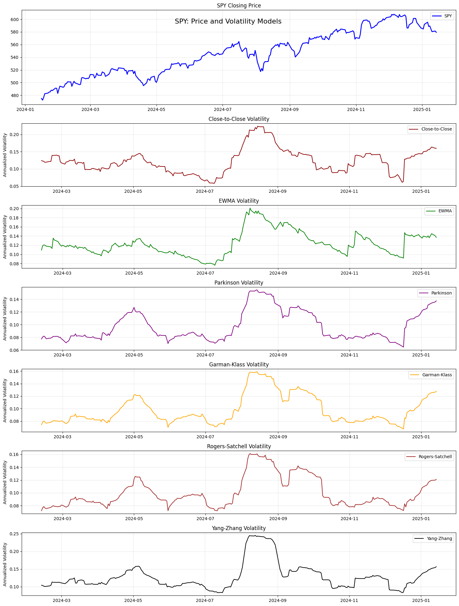
Volatility modelling is fundamental to financial analysis and risk management. Different models have been developed over time to capture various aspects of price movements and market behaviour. This guide explores the major volatility models, their mathematical foundations, and practical applications.
You will have every model written in Python as you read this;
The full end-to-end workflow is available in a Google Colab notebook, exclusively for paid subscribers of my newsletter. Paid subscribers also gain access to the complete article, including the full code snippet in the Google Colab notebook, which is accessible below the paywall at the end of the article. Subscribe now to unlock these benefits!
First, let´s import the libraries and $SPY prices:
import numpy as np
import pandas as pd
import yfinance as yf
from datetime import datetime, timedelta
import matplotlib.pyplot as plt

plt.style.use('default')
pd.set_option('display.max_columns', None)


def get_spy_data():
    """
    Retrieves SPY data for the last year using yfinance.
    Returns a DataFrame with Open, High, Low, Close prices.
    """
    end_date = datetime.now()
    start_date = end_date - timedelta(days=365)

    spy = yf.download('SPY', start=start_date, end=end_date)
    return spy
Close-to-Close Volatility Model
Tackle your credit card debt by paying 0% intro APR until 2027
Pay introductory no interest until 2027 with some of the best hand-picked credit cards this year. They are perfect for anyone looking to pay down their debt, and not add to it!
Click here to see what all of the hype is about.
Overview
The close-to-close volatility model is the most traditional and widely used approach. It uses daily closing prices to estimate volatility, making it particularly reliable due to the high liquidity typically present during closing auctions.
Mathematical Formula
The close-to-close volatility is calculated as:
σcc = √[F/(N-1)] × √[∑(xi — x̄)²]
Where:
- σcc = Close-to-close volatility
- F = Annualization factor (252 for daily data)
- N = Number of observations
- xi = ln(ci/ci-1) = logarithmic return
- ci = Closing price at time i
- x̄ = Mean of logarithmic returns (often assumed to be zero)
Strengths and Limitations
Strengths:
- Uses reliable closing prices from liquid market periods
- Simple to calculate and widely understood
- Most appropriate for variance swap pricing
Limitations:
- Ignores intraday price movements
- May miss significant volatility between closing periods
- Requires more data points for accurate estimation
def calculate_close_to_close(data, window=20):
    """
    Calculates Close-to-Close volatility.
    This is the traditional method using only closing prices.

    Parameters:
        data: DataFrame with price data
        window: Rolling window size for calculation

    Returns:
        Annualized volatility series
    """
    returns = np.log(data['Close'] / data['Close'].shift(1))
    vol = np.sqrt(252) * returns.rolling(window=window).std(ddof=1)
    return vol
Exponentially Weighted Volatility Model
Overview
This model assigns more weight to recent observations, making it more responsive to current market conditions while still maintaining historical context.
Mathematical Formula
σt² = λσt-¹² + (1-λ)xt²
Where:
- σt = Volatility at time t
- λ = Decay factor (typically around 0.94 for daily data)
- xt = Return at time t
Strengths and Limitations
Strengths:
- More responsive to recent market changes
- Smoother transitions in volatility estimates
- Helps prevent volatility estimate collapse
Limitations:
- Sensitive to parameter choice (λ)
- May not handle regular events (like earnings) well
- Can overreact to recent extreme events
def calculate_ewma(data, window=20, lambda_param=0.94):
    """
    Calculates Exponentially Weighted Moving Average volatility.
    This method gives more weight to recent observations.

    Parameters:
        data: DataFrame with price data
        window: Initial window size for calculation
        lambda_param: Decay factor (typically 0.94 for daily data)

    Returns:
        Annualized EWMA volatility series
    """
    returns = np.log(data['Close'] / data['Close'].shift(1))
    returns = returns.fillna(0)

    vol = pd.Series(np.nan, index=returns.index)
    vol.iloc[window-1] = np.sqrt(252) * returns.iloc[:window].std(ddof=1)

    for i in range(window, len(returns)):
        if np.isnan(vol.iloc[i-1]):
            vol.iloc[i] = np.sqrt(252) * returns.iloc[i-window:i].std(ddof=1)
        else:
            vol.iloc[i] = np.sqrt(252 * ((1 - lambda_param) * returns.iloc[i]**2 +
                                        lambda_param * (vol.iloc[i-1]/np.sqrt(252))**2))

    return vol
Parkinson Model (High-Low)
Overview
Developed by Michael Parkinson in 1980, this model…
Subscribe to our premium content to read the rest.
Become a paying subscriber to get access to this post and other subscriber-only content.
Upgrade


