In partnership with

The Volatility Cone: A Quant's Tool for Mapping Price Uncertainty

Here’s your lifeline.

Another headline. Another client pays late. The next 10 days shift. You open your bank app before walking into the office.

The hits just keep coming right now.

And as the leader, you’re the one absorbing all of them.

But survival doesn’t come from holding tighter alone.

The Small Business Survivor Guide gives you 83 practical ways to cut costs, stabilize cash flow, and navigate economic pressure with confidence.

Because in times like these, stability isn’t luck. It’s strategy.

And the leaders who stay standing are the ones who prepare for what’s next.

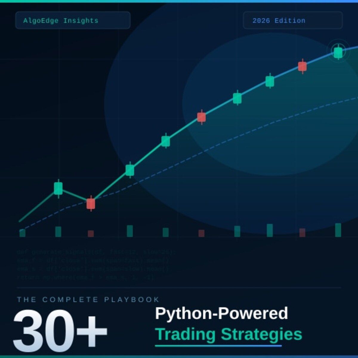
② One strategy in this book returned 2.3× the S&P 500 on a risk-adjusted basis over 5 years.

Fully coded in Python. Yours to run today.

The 2026 Playbook — 30+ backtested strategies,
full code included, ready to deploy.

20% off until Tuesday. Use APRIL2026 at checkout.

$79 → $63.20 · Expires April 7.

→ Grab it before Tuesday

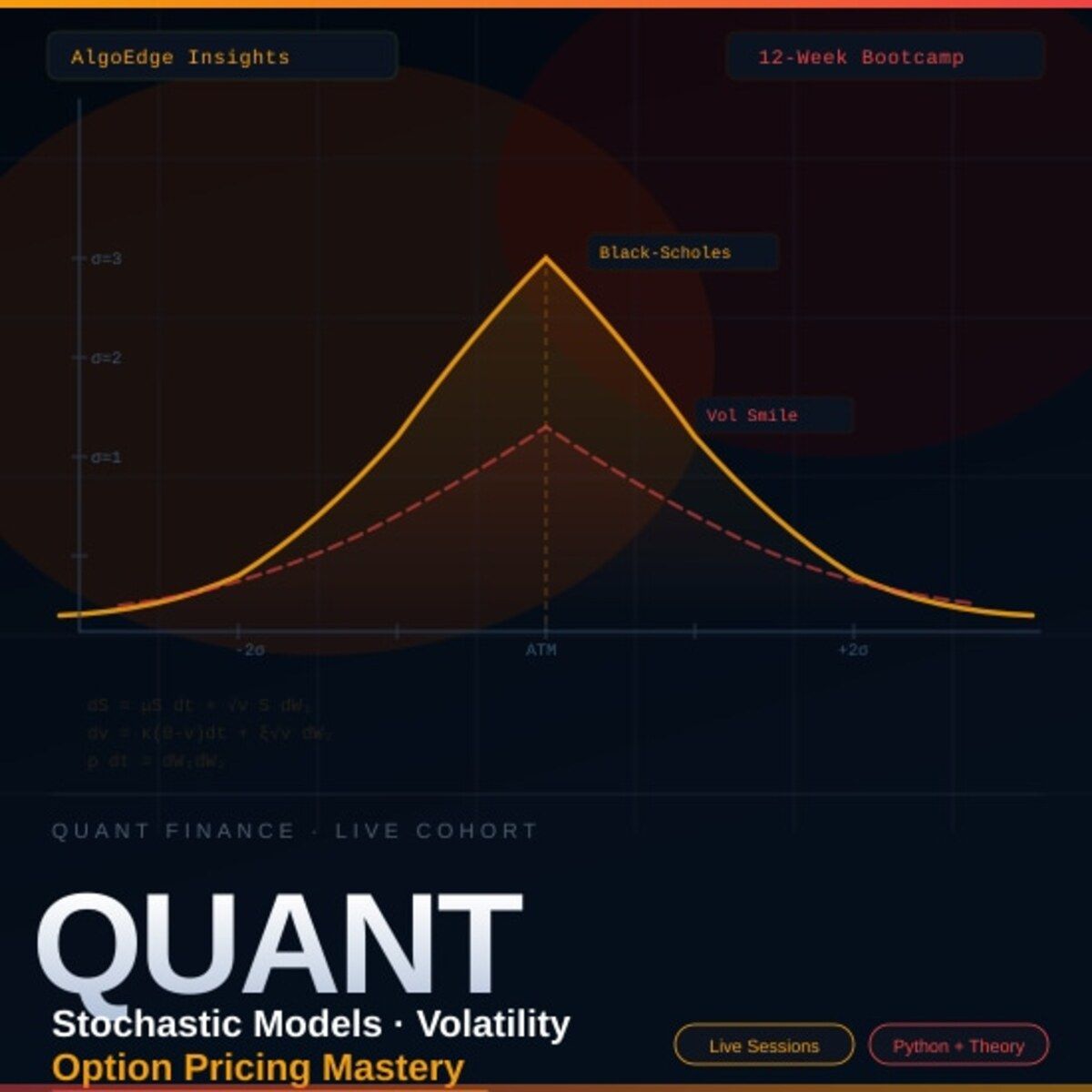
⑤ Most quant courses teach you to watch. This one makes you build.

Live. Weekly. With feedback on your actual code.

The AlgoEdge Quant Finance Bootcamp — 12 weeks of stochastic models, Black-Scholes, Heston, volatility surfaces, and exotic options. Built from scratch in Python.

Not pre-recorded. Not self-paced. Live sessions, weekly homework, direct feedback, and a full code library that's yours to keep.

Cohort size is limited intentionally — so every question gets answered.

→ Before you enroll, reach out for a 15-minute fit check. No pitch, no pressure.

📩 Email first: [email protected]

Premium Members – Your Full Notebook Is Ready

The complete Google Colab notebook from today’s article (with live data, full Hidden Markov Model, interactive charts, statistics, and one-click CSV export) is waiting for you.

Preview of what you’ll get:

Inside the Strategy Lab

  • 📥 Auto-fetches cross-asset market data — Pulls SPY, IWM, HYG, LQD, and VIX price history from Yahoo Finance and aligns everything into one unified dataframe.

  • 🧮 Feature engineering pipeline — Builds credit spread, daily/21D/63D/126D returns, relative SPY vs IWM returns, realized volatility, VIX transformations, and drawdown features.

  • ⚖️ Volatility context logic — Compares implied volatility to realized volatility using VIX-to-SPX volatility ratios and rolling VIX averages to help spot regime shifts.

  • 🧼 Data cleaning step — Removes rows with missing or infinite values before modeling so the clustering and PCA steps run on clean input only.

  • 📐 Standardization + PCA — Scales all numeric features, then compresses them with PCA while keeping enough components to explain 95% of the variance.

  • 🔍 Silhouette-based cluster search — Tests multiple K-Means cluster counts and picks the best number using silhouette score on both raw and PCA-reduced features.

  • 🧠 Regime classification output — Assigns a regime label to each valid row and stores it back into the main dataframe as a nullable integer column.

  • 📊 Price and cluster visualization — Generates an OHLCV chart for SPY and a PCA scatter plot colored by detected regime.

  • 📈 Model quality reporting — Prints the number of rows used, best silhouette scores, chosen representation, and final regime distribution.

Free readers – you already got the full breakdown and visuals in the article. Paid members – you get the actual tool.

Not upgraded yet? Fix that in 10 seconds here👇

Google Collab Notebook With Full Code Is Available In the End Of The Article Behind The Paywall 👇 (For Paid Subs Only)

Welcome to Part 1 of Hybrid Machine Learning for Market Regime Detection in Python! 👋

In Part 1, we concentrate on SPY, IWM, HYG, LQD, and VIX as the core instruments of our analysis. These instruments were picked because they they form a compact, cross-asset snapshot of market risk appetite, liquidity conditions, and volatility expectations, viz.

  • SPY tracks the S&P 500 and represents large-cap U.S. equities (benchmark risk-on/risk-off sentiment)

  • IWM tracks small-cap U.S. stocks (higher beta and risk appetite)

  • HYG represents lower-rated corporate debt (indicator of financial stress)

  • LQD helps separate liquidity stress from macro rate-driven shifts

  • VIX represents expected volatility (fear gauge) and captures tail-risk pricing.

Rhetorical question:

Markets are often said to run on supply and demand, and that supply and demand are ultimately driven by investors’ emotions, beliefs, and reactions. While technology and and society look very different from decades ago, human psychology has not changed nearly as much.

By uncovering a fundamental paradox at the heart of market uncertainty, this post demonstrates that market regime detection can distinguish between different states of complex price dynamics and shed light on repeated forecasting failures, even if it cannot fully prevent them.

Here are the main ideas guiding our methodology throughout this study:

  • Data sources like EODHD APIs (with a 10% discount) are important for robust regime detection because regime models are only as good as the data feeding them. Detecting structural shifts in markets (volatility spikes, correlation breakdowns, liquidity contractions, macro cycles, etc.) requires depth, consistency, and reliability in historical and real time data. To identify these patterns, we need clean, long term historical data across multiple market environments, including crises and expansions. Sparse or short datasets make regime segmentation unreliable.

  • In the fast-moving world of quantitative finance, unsupervised learning has become a handy tool for uncovering hidden patterns and connections in market data. Unsupervised machine learning (ML) techniques include Agglomerative, K-Means clustering, and Gaussian Mixture Models. In this article, we focus on the K-Means clustering technique due to its simplicity and efficiency [1–3]. Because market behavior changes across regimes, K-Means groups similar historical data together, making hidden market states easier to spot.

  • After that, supervised ML [6–8] lets us classify/rank the market states for unseen data, based on past data labeled with K-Means clusters. This is commonly referred to as a hybrid approach to detecting regime switches in financial markets. It has been shown that the results of the ML classification can be used to develop a trading strategy for a market-on-open order that is informed by historical market fluctuations.

  • Finally, in market regime detection, it’s not enough to just know which regime the market is in, we also want to understand why. That’s where Interpretable Machine Learning (IML) comes in, helping us see which factors are driving the predictions and making the results easier to trust and act on [4, 5, 9] (read more here).

Let’s get to the heart of the matter! 🚀

Contents

· Step 1: Reading Tradable Instruments
· Step 2: Preparing Data for ML Training
· Step 3: PCA, K-Means Clusters & QC
· Step 4: ML Classification & Cross-Validation
· Step 5: Interpretable Machine Learning
· Conclusions
· References 📚

Your ads ran overnight. Nobody was watching. Except Viktor.

One brand built 30+ landing pages through Viktor without a single developer.

Each page mapped to a specific ad group. All deployed within hours. Viktor wrote the code and shipped every one from a Slack message.

That same team has Viktor monitoring ad accounts across the portfolio and posting performance briefs before the day starts. One colleague. Always on. Across every account.

Step 1: Reading Tradable Instruments

We will use the EODHD APIs to retrieve daily historical data for SPY.US (the SPDR S&P 500 ETF, a widely traded U.S. large-cap equity ETF), IWM.US (the iShares Russell 2000 ETF, a widely used small-cap equity ETF in the U.S. market), HYG.US (the iShares High-Yield Corporate Bond ETF, commonly used as a proxy for credit risk in regime analysis), LQD.US (the iShares Investment-Grade Corporate Bond ETF, widely used as a benchmark for safer corporate credit exposure), and VIX.VN (Market Volatility / Risk Sentiment Indicator) spanning 2021–01–04 to 2026–02–20

import pandas as pd
import numpy as np
import matplotlib.pyplot as plt
from eodhd import APIClient
import requests
import mplfinance as mpf

API_KEY = "64469ca80bd5a1.03505250"   # your EODHD API key


start_date = "2021-01-04"
end_date = "2026-02-20"


def fetch_eod(symbol, start_date, end_date):
    """
    Fetch EOD data for a given symbol from EODHD.
    """
    url = f"https://eodhd.com/api/eod/{symbol}"
    params = {
        "api_token": API_KEY,
        "from": start_date,
        "to": end_date,
        "fmt": "json"
    }
    resp = requests.get(url, params=params)
    data = resp.json()
    df = pd.DataFrame(data)
    df = df.sort_values("date")
    df["date"] = pd.to_datetime(df["date"])
    df.set_index("date", inplace=True)
    return df

# Fetch SPY and IWM EOD data
spy_df = fetch_eod("SPY.US", start_date, end_date)
iwm_df = fetch_eod("IWM.US", start_date, end_date)
hyg_df = fetch_eod("HYG.US", start_date, end_date)
lqd_df = fetch_eod("LQD.US", start_date, end_date)
symbol = "VIX.VN"
vix_df=fetch_eod(symbol, start_date, end_date)

spy_df.tail()

           open         high         low          close        adjusted_close volume
date      
2026-02-13 681.69000000 686.28000000 677.52000000 681.75000000 681.75000000 96267500
2026-02-17 680.14000000 684.94000000 675.78000000 682.85000000 682.85000000 81354700
2026-02-18 684.02000000 689.15000000 682.83000000 686.29000000 686.29000000 73570300
2026-02-19 683.84000000 686.18000000 681.55000000 684.48000000 684.48000000 58649400
2026-02-20 682.32000000 690.00000000 681.73000000 689.43000000 689.43000000 99309328

spy_df.info()

<class 'pandas.core.frame.DataFrame'>
DatetimeIndex: 1289 entries, 2021-01-04 to 2026-02-20
Data columns (total 6 columns):
 #   Column          Non-Null Count  Dtype  
---  ------          --------------  -----  
 0   open            1289 non-null   float64
 1   high            1289 non-null   float64
 2   low             1289 non-null   float64
 3   close           1289 non-null   float64
 4   adjusted_close  1289 non-null   float64
 5   volume          1289 non-null   int64  
dtypes: float64(5), int64(1)
memory usage: 70.5 KB
  • Using Plotly to create OHLC & Volume charts of these trading instruments

import plotly.graph_objects as go
from plotly.subplots import make_subplots
import pandas as pd

# Make sure datetime index
df_plot = spy_df.copy()
#df_plot.index = pd.to_datetime(spy_df.index)

# Create subplots: 2 rows, shared x-axis
fig = make_subplots(
    rows=2, cols=1,
    shared_xaxes=True,
    row_heights=[0.7, 0.3],   # 70% candlestick, 30% volume
    vertical_spacing=0.02
)

# Add OHLC candlestick trace in row 1
fig.add_trace(go.Candlestick(
    x=spy_df.index,
    open=df_plot['open'],
    high=df_plot['high'],
    low=df_plot['low'],
    close=df_plot['close'],
    name='OHLC',
    increasing_line_color='green',
    decreasing_line_color='red'
), row=1, col=1)

# Add volume bar trace in row 2
fig.add_trace(go.Bar(
    x=spy_df.index,
    y=df_plot['volume'],
    name='Volume',
    marker_color='darkblue',
    opacity=1
), row=2, col=1)

# Layout
fig.update_layout(
    title='SPY OHLC Candlestick with Volume Below',
    xaxis1=dict(rangeslider_visible=False),
    xaxis2=dict(title='Date'),
    yaxis1=dict(title='Price'),
    yaxis2=dict(title='Volume'),
    template='ggplot2',
    width=1000,
    height=600,
    legend=dict(orientation='h', yanchor='bottom', y=1.02, xanchor='right', x=1)
)

fig.show()

SPY OHLC Candlestick with Volume Below

IWM OHLC Candlestick with Volume Below

HYG OHLC Candlestick with Volume Below

LQD OHLC Candlestick with Volume Below

VIX.VN OHLC Candlestick with Volume Below

Qualitative Interpretation of 2021–2026 Cycle

  • A joint regime interpretation of the above trading instruments gives a much cleaner regime classification than SPY alone because we capture equity beta dispersion (SPY vs IWM), credit stress (HYG vs LQD), volatility clustering (VIX), and duration sensitivity (LQD).

  • 2021 was a smooth liquidity-driven melt-up: SPDR S&P 500 ETF Trust, iShares Russell 2000 ETF, and iShares iBoxx $ High Yield Corporate Bond ETF were all trending higher, iShares iBoxx $ Investment Grade Corporate Bond ETF was stable, and the CBOE Volatility Index stayed low.

  • 2022 was a full tightening shock: SPDR S&P 500 ETF Trust fell, iShares Russell 2000 ETF got hit even harder, iShares iBoxx $ High Yield Corporate Bond ETF and iShares iBoxx $ Investment Grade Corporate Bond ETF both dropped, and the CBOE Volatility Index stayed elevated as rates crushed everything at once.

  • 2023 was a narrow recovery: SPDR S&P 500 ETF Trust pushed higher while iShares Russell 2000 ETF, iShares iBoxx $ High Yield Corporate Bond ETF, and iShares iBoxx $ Investment Grade Corporate Bond ETF mostly chopped sideways, with the CBOE Volatility Index drifting lower.

  • 2024 was a broad expansion: SPDR S&P 500 ETF Trust, iShares Russell 2000 ETF, iShares iBoxx $ High Yield Corporate Bond ETF, and iShares iBoxx $ Investment Grade Corporate Bond ETF were all trending higher together while the CBOE Volatility Index stayed low.

  • 2025 feels late-cycle: SPDR S&P 500 ETF Trust is still grinding higher, iShares Russell 2000 ETF is lagging, iShares iBoxx $ High Yield Corporate Bond ETF is flat, iShares iBoxx $ Investment Grade Corporate Bond ETF is rate-sensitive, and the CBOE Volatility Index is compressed but vulnerable.

  • 2026 looks like an inflection year — watch iShares Russell 2000 ETF as the leading indicator, a potential credit pivot in iShares iBoxx $ High Yield Corporate Bond ETF, a duration pivot in iShares iBoxx $ Investment Grade Corporate Bond ETF, and rising regime-shift risk for SPDR S&P 500 ETF Trust.

Find out more here:

Step 2: Preparing Data for ML Training

Let’s compute several extra features [1] for use in both unsupervised and supervised ML models: credit spread, rolling windowed returns (1D, 21D, 63D, 126D), the 3‑ and 6‑month moving averages of VIX, and the key ratios, measuring whether implied volatility (VIX) is above or below recent actual volatility:

  • Calculating the logarithmic spread between high-yield (HYG) and investment-grade (LQD) bond prices

df=spy_df.copy()
# Credit Spread (proxy)
df["Credit_Spread"] = np.log(hyg_df['adjusted_close']) - np.log(lqd_df['adjusted_close'])
  • These lines calculate SPY and IWM instant returns over different time windows, from daily to 6 months, which are often used as features in momentum analysis

# SPY Returns
df["SPX_Daily_Return"]  = spy_df['close'].pct_change()
df["SPX_21D_Return"]    = spy_df['close'].pct_change(21)
df["SPX_63D_Return"]    = spy_df['close'].pct_change(63)
df["SPX_126D_Return"]   = spy_df['close'].pct_change(126)

# IWM Returns

df["RUT_Daily_Return"]  = iwm_df['close'].pct_change()
df["RUT_21D_Return"]    = iwm_df['close'].pct_change(21)
df["RUT_63D_Return"]    = iwm_df['close'].pct_change(63)
df["RUT_126D_Return"]   = iwm_df['close'].pct_change(126)
  • This calculates the relative performance of the S&P 500 (SPY) versus the Russell 2000 (IWM) over the past 21 trading days

# Relative performance SPX vs Russell (large vs small caps)
df["SPX_vs_RUT_21D"] = df["SPX_21D_Return"] - df["RUT_21D_Return"]
df["SPX_vs_RUT_63D"] = df["SPX_63D_Return"] - df["RUT_63D_Return"]
  • Calculating the rolling standard deviation of our return series over a fixed window (default 21 days)

# Realized Volatility
def realized_vol(series, window=21, trading_days=252):
    return series.rolling(window).std() * np.sqrt(trading_days)

#computes historical (actual) volatility of a return series over a rolling window
#Volatility measures how much the price fluctuates over a period
#annualized (×sqrt(252) for daily returns) to compare across periods

df["SPX_21D_RealVol"] = realized_vol(df["SPX_Daily_Return"], window=21) #Captures short-term fluctuations 
df["SPX_63D_RealVol"] = realized_vol(df["SPX_Daily_Return"], window=63) #Useful for medium-term risk assessment
df["RUT_21D_RealVol"] = realized_vol(df["RUT_Daily_Return"], window=21)
df["RUT_63D_RealVol"] = realized_vol(df["RUT_Daily_Return"], window=63)

'''
Comparing SPY vs RUT realized vol helps detect regime shifts: e.g., 
when small caps get riskier than large caps.

Short vs medium-term realized vol gives insight into volatility clustering, 
which is critical for risk management, position sizing, and ML models.
'''
  • Calculating a smoothed, 3-month equivalent VIX, ready to compare against current VIX levels for feature engineering

# Compute vix3m_close
df['vix3m_close'] = vix_df['close'] * np.sqrt(3)

# Fill NaNs with nearest values (forward then backward)
df['vix3m_close'] = df['vix3m_close'].fillna(method='ffill').fillna(method='bfill')

# Compute rolling 3-month (63 trading days) average
df['vix3m_rolling_avg'] = df['vix3m_close'].rolling(window=63, min_periods=1).mean()

# Now vix_df['vix3m_rolling_avg'] contains the rolling 3-month average
  • The same steps apply for a 6-month average: we scale the VIX by sqrt(6) to get a 6-month volatility equivalent, fill any missing values forward and backward to ensure a complete series, and then compute a 126-day rolling average to smooth it, resulting in vix6m_rolling_avg for medium-term volatility trends

# Compute vix6m_close
df['vix6m_close'] = vix_df['close'] * np.sqrt(6)

# Step 2: Fill NaNs with nearest values (forward then backward)
df['vix6m_close'] = df['vix6m_close'].fillna(method='ffill').fillna(method='bfill')

# Step 3: Compute rolling 6-month (126 trading days) average
df['vix6m_rolling_avg'] = df['vix6m_close'].rolling(window=126, min_periods=1).mean()

# Now vix_df['vix6m_rolling_avg'] contains the rolling 6-month average
  • Determining the daily and weekly changes in VIX to highlight short-term spikes or drops in implied volatility

df["VIX_1D_Change"]     = vix_df["close"].diff(1)
df["VIX_5D_Change"]     = vix_df["close"].diff(5)
  • Computing the ratio of current VIX to the 21-day realized volatility of the S&P 500

df["VIX_to_SPXRealVol"] = vix_df["close"] / df["SPX_21D_RealVol"]

#When implied volatility is higher than realized volatility, it usually means the options market is bracing for more risk.
#When VIX is below actual realized volatility, it usually means the market is feeling a bit too relaxed.
  • Comparing the 3-month rolling average of VIX to the current VIX

df["VIX3M_VIX"] = df["vix3m_rolling_avg"] / vix_df["close"]

#Helps detect whether VIX is high or low relative to recent volatility trends.

#Useful for spotting volatility spikes or regime shifts.
  • Same idea, but over 6 months (medium-term trend)

df["VIX6M_VIX"] = df["vix6m_rolling_avg"] / vix_df["close"]

#Provides a longer-term context to current volatility levels, which is helpful for trend vs mean-reversion analysis.
  • Computing drawdowns by measuring how far the current price has fallen from its 6-month high, viz.

Drawdown = (Current Price)/(Rolling Max) — 1

# Drawdowns
spx_roll_max = spy_df["close"].rolling(126, min_periods=1).max()
rut_roll_max = iwm_df["close"].rolling(126, min_periods=1).max()
df["SPX_126D_Drawdown"] = spy_df["close"] / spx_roll_max - 1.0
df["RUT_126D_Drawdown"] = iwm_df["close"] / rut_roll_max - 1.0

#A drawdown of 0 means the price is at its 6-month high, while a negative value shows how far it has fallen below that peak 
# e.g., -0.10 = 10% drop

#Useful for identifying corrections, market stress, and risk-on/risk-off regimes
  • Cleaning up the DataFrame by removing all rows that contain any missing values (NaNs) and then resetting the row index so it runs sequentially from 0 again

df = df.dropna().reset_index(drop=True)
  • Checking the general structure of this DataFrame

df.info()

<class 'pandas.core.frame.DataFrame'>
RangeIndex: 1116 entries, 0 to 1115
Data columns (total 32 columns):
 #   Column             Non-Null Count  Dtype  
---  ------             --------------  -----  
 0   open               1116 non-null   float64
 1   high               1116 non-null   float64
 2   low                1116 non-null   float64
 3   close              1116 non-null   float64
 4   adjusted_close     1116 non-null   float64
 5   volume             1116 non-null   int64  
 6   Credit_Spread      1116 non-null   float64
 7   SPX_Daily_Return   1116 non-null   float64
 8   SPX_21D_Return     1116 non-null   float64
 9   SPX_63D_Return     1116 non-null   float64
 10  SPX_126D_Return    1116 non-null   float64
 11  RUT_Daily_Return   1116 non-null   float64
 12  RUT_21D_Return     1116 non-null   float64
 13  RUT_63D_Return     1116 non-null   float64
 14  RUT_126D_Return    1116 non-null   float64
 15  SPX_vs_RUT_21D     1116 non-null   float64
 16  SPX_vs_RUT_63D     1116 non-null   float64
 17  SPX_21D_RealVol    1116 non-null   float64
 18  SPX_63D_RealVol    1116 non-null   float64
 19  RUT_21D_RealVol    1116 non-null   float64
 20  RUT_63D_RealVol    1116 non-null   float64
 21  vix3m_close        1116 non-null   float64
 22  vix3m_rolling_avg  1116 non-null   float64
 23  vix6m_close        1116 non-null   float64
 24  vix6m_rolling_avg  1116 non-null   float64
 25  VIX_1D_Change      1116 non-null   float64
 26  VIX_5D_Change      1116 non-null   float64
 27  VIX_to_SPXRealVol  1116 non-null   float64
 28  VIX3M_VIX          1116 non-null   float64
 29  VIX6M_VIX          1116 non-null   float64
 30  SPX_126D_Drawdown  1116 non-null   float64
 31  RUT_126D_Drawdown  1116 non-null   float64
dtypes: float64(31), int64(1)
memory usage: 279.1 KB
  • Creating a full EDA profiling report and saving it as an HTML file (see details in Appendix A)

import pandas_profiling

# Generate a profiling report
profile = pandas_profiling.ProfileReport(df, title="DataFrame Profiling Report", explorative=True)

# Export as HTML
profile.to_file("df_profiling_report.html")
  • Backing up the feature engineering above with simple Pandas visualizations in Appendix B.

Step 3: PCA, K-Means Clusters & QC

Let’s apply PCA for dimensionality reduction on the engineered features, followed by K-Means clustering and using the Silhouette score for quality control [1–3].

  • Building a clean feature matrix for modeling by automatically selecting only the relevant numeric features and excluding raw/helper columns

df["spx_close"]=spy_df['close']
df["rut_close"]=iwm_df['close']

exclude_exact = {
    "date",
    "spx_close", "rut_close",     # raw prices
    "HYG", "LQD",                 # raw ETF prices 
    "SPX_50D_MA", "SPX_200D_MA",  # helper MAs
    "vix3m_close", "vix6m_close", # raw VIX maturities
}
numeric_cols = df.select_dtypes(include=[np.number]).columns.tolist()
feature_cols = [c for c in numeric_cols if c not in exclude_exact]
  • Standardizing the features ensures they all contribute equally by setting the mean to 0 and the standard deviation to 1, resulting in more consistent and meaningful regime clustering

88% resolved. 22% loyal. Your stack has a problem.

Those numbers aren't a CX issue — they're a design issue. Gladly's 2026 Customer Expectations Report breaks down exactly where AI-powered service loses customers, and what the architecture of loyalty-driven CX actually looks like.

from sklearn.preprocessing import StandardScaler
# Clean (drop inf/NaN rows across features), keep index map
X_df = df[feature_cols].replace([np.inf, -np.inf], np.nan).dropna()
valid_idx = X_df.index

# Standardize
scaler = StandardScaler()
X_scaled = scaler.fit_transform(X_df.values)

print(f"Using {len(feature_cols)} features on {len(valid_idx)} rows.")
print("Example (first row, scaled):")
print(dict(zip(feature_cols, X_scaled[0])))

Using 30 features on 1111 rows.
Example (first row, scaled):
{'open': -0.6951180345351432, 'high': -0.7229587830574913, 'low': -0.703917059716172, 'close': -0.7053736085571439, 'adjusted_close': -0.7930558463267813, 'volume': -0.25193827116749395, 'Credit_Spread': -1.920316446670385, 'SPX_Daily_Return': -0.20888694633192142, 'SPX_21D_Return': 0.3264870523513826, 'SPX_63D_Return': 0.5441734122659411, 'SPX_126D_Return': 1.1374491121799157, 'RUT_Daily_Return': -1.0242951987900164, 'RUT_21D_Return': -0.19670212834312645, 'RUT_63D_Return': -0.04251714529713277, 'RUT_126D_Return': 1.3294014066194912, 'SPX_vs_RUT_21D': 0.7716287518912586, 'SPX_vs_RUT_63D': 0.9240644053970356, 'SPX_21D_RealVol': -0.8163409650641269, 'SPX_63D_RealVol': -0.7911947901693893, 'RUT_21D_RealVol': -0.7535218830599567, 'RUT_63D_RealVol': -0.7646578687379872, 'vix3m_rolling_avg': 1.8531365214563946, 'vix6m_rolling_avg': 2.0004951059030094, 'VIX_1D_Change': -2.6441344294254545, 'VIX_5D_Change': -1.6846822958712968, 'VIX_to_SPXRealVol': 1.4593656676971463, 'VIX3M_VIX': 0.38894073787556366, 'VIX6M_VIX': 0.17508794656773055, 'SPX_126D_Drawdown': 0.7685136183378205, 'RUT_126D_Drawdown': 0.7028769490114624}
  • Remark: the line X_scaled = scaler.fit_transform(X_df.values) could introduce look ahead bias if the data is later split into train and test sets based on time. In this case, though, the code is only used for clustering on the full historical dataset. We are not training a predictive model or running a trading simulation. Still, to be on the safe side and avoid any potential leakage, this line can be replaced with an expanding (walk forward) standardization approach, which is commonly used in time series models to prevent look ahead bias (see Appendix C).

  • Performing PCA on the standardized features, transforming them into a smaller set of uncorrelated components that capture most of the variance, which is useful for clustering

# PCA reduction (variance target)
from sklearn.decomposition import PCA #Imports Principal Component Analysis (PCA) from scikit-learn
variance_target = 0.95 #use it later to decide how many components to keep
pca = PCA()
X_pca = pca.fit_transform(X_scaled)
explained_var = pca.explained_variance_ratio_

plt.figure(figsize=(8,5))
plt.plot(np.cumsum(explained_var), marker="o")
plt.xlabel("Number of Principal Components")
plt.ylabel("Cumulative Explained Variance")
plt.title("PCA - Cumulative Variance Explained")
plt.grid(True)
plt.show()

#PCA is used to reduce the dimensionality of a dataset while retaining most of the variance (information).

PCA — Cumulative Variance Explained

  • Determining the number of components to retain

from sklearn.cluster import KMeans
from sklearn.metrics import silhouette_score
#https://farshadabdulazeez.medium.com/understanding-silhouette-score-in-clustering-8aedc06ce9c4

n_components = np.argmax(np.cumsum(explained_var) >= variance_target) + 1

#Retain enough components to capture the desired proportion of variance, while discarding less informative dimensions.
  • Reducing the PCA-transformed data by selecting only the first n_components columns of X_pca

X_pca_reduced = X_pca[:, :n_components]
print(f"Selected {n_components} PCs (≈{np.cumsum(explained_var)[n_components-1]:.3f} variance)")

Selected 13 PCs (≈0.962 variance)

'''
Reduces noise and redundancy.

Speeds up clustering or other ML algorithms.

Keeps most of the important information while simplifying the feature space
'''
  • Defining the function [1]

def silhouette_over_k(X, k_min=2, k_max=6, seed=42):
    scores = {}
    for k in range(k_min, k_max+1):
        km = KMeans(n_clusters=k, n_init=50, random_state=seed)
        labels = km.fit_predict(X)
        scores[k] = silhouette_score(X, labels)
    return scores

This function takes a dataset X, which can be either the raw scaled features or the PCA-reduced features. We also provide a minimum k_min and maximum k_max number of clusters to try, as well as a seed to ensure reproducible results. For each value of k in the specified range, the function initializes a K-Means model with k clusters and 50 random initializations, fits the model to the data, and computes cluster labels. It then calculates the Silhouette score, which ranges from -1 to 1 and indicates how well each point fits within its cluster compared to other clusters. Scores close to 1 mean the clusters are well-separated, scores around 0 indicate overlapping clusters, and negative scores suggest points may be assigned to the wrong cluster [3]. The function returns a dictionary mapping each k to its corresponding Silhouette score.

  • Running on raw vs PCA data

scores_raw = silhouette_over_k(X_scaled, 2, 6) #silhouette scores for clusters 2–6 on scaled features
scores_pca = silhouette_over_k(X_pca_reduced, 2, 6) #silhouette scores for clusters 2–6 on PCA-reduced features

print("\nSilhouette (raw scaled):", {k: round(v,3) for k,v in scores_raw.items()})
print("Silhouette (PCA reduced):", {k: round(v,3) for k,v in scores_pca.items()})

Silhouette (raw scaled): {2: 0.224, 3: 0.182, 4: 0.184, 5: 0.176, 6: 0.173}
Silhouette (PCA reduced): {2: 0.233, 3: 0.191, 4: 0.173, 5: 0.186, 6: 0.183}

'''

Allows you to compare clustering quality before and after dimensionality reduction.

PCA often improves cluster separation by removing noise and correlated features.

Silhouette scores help choose the optimal number of clusters (highest score).
'''

This snippet evaluates K-Means clustering quality across different numbers of clusters for both the full feature set and the PCA-reduced set, using the Silhouette score to identify the best representation and cluster count.

  • Finding the best number of clusters for each representation and deciding which representation to use

# Choose representation with higher best silhouette
best_k_raw = max(scores_raw, key=scores_raw.get)
best_k_pca = max(scores_pca, key=scores_pca.get)

use_pca = scores_pca[best_k_pca] >= scores_raw[best_k_raw]
rep = "PCA" if use_pca else "RAW"
best_k = best_k_pca if use_pca else best_k_raw
X_final = X_pca_reduced if use_pca else X_scaled

print(f"\nChose {rep} features with k={best_k} "
      f"(silhouette={max(scores_pca.values()) if use_pca else max(scores_raw.values()):.3f})")

Chose PCA features with k=2 (silhouette=0.233)

'''

Compares the best Silhouette scores from both representations.

If PCA’s score is equal to or higher than raw features, it chooses PCA; otherwise, it keeps the raw features.

rep is a string indicating which representation was selected ("PCA" or "RAW").

best_k is the optimal number of clusters based on the selected representation.

X_final is the dataset that will be used for clustering (either X_pca_reduced or X_scaled).
'''

This snippet automatically picks the most meaningful feature representation for clustering. It ensures the clusters are as well-separated as possible according to the Silhouette score. Overall, it simplifies downstream modeling by selecting both the best dataset and best number of clusters.

  • Initializing K-Means, fitting the model and assigning cluster labels

# Fit final KMeans on chosen representation
kmeans = KMeans(n_clusters=best_k, n_init=50, random_state=42)
final_labels = kmeans.fit_predict(X_final)
'''
n_clusters=best_k use the optimal number of clusters determined from the Silhouette analysis
n_init=50 run K-Means 50 times with different random starting points and pick the best result to avoid poor local minima
random_state=42 ensures reproducible results

final_labels contains the cluster assignments for every observation in our dataset
'''

These labels can now be used for market regime classification. By using the best representation and optimal cluster count, the clustering is as meaningful and stable as possible.

  • Creating a Regime column and filling it with the K-Means cluster labels for valid rows (ensure it’s stored as a clean nullable integer column)

# Write labels back to original df (only rows used after cleaning)
df["Regime"] = np.nan
df.loc[valid_idx, "Regime"] = final_labels
df["Regime"] = df["Regime"].astype("Int64")  # nullable int

print("\nRegime distribution (on modeled rows):")
print(pd.Series(final_labels).value_counts().sort_index())

Regime distribution (on modeled rows):
0    662
1    449
Name: count, dtype: int64

Top loadings for PC1:
SPX_21D_RealVol     -0.23146125
SPX_63D_RealVol     -0.20523070
RUT_21D_RealVol     -0.19656260
RUT_63D_RealVol     -0.18900041
VIX6M_VIX           -0.17146740
VIX3M_VIX           -0.14419710
volume              -0.13314339
SPX_vs_RUT_63D      -0.07062695
SPX_63D_Return       0.23360656
open                 0.23440299
close                0.23505144
low                  0.23681908
RUT_126D_Return      0.25053307
SPX_126D_Return      0.25384981
SPX_126D_Drawdown    0.26048314
RUT_126D_Drawdown    0.26416006
Name: PC1, dtype: float64

Top loadings for PC2:
SPX_vs_RUT_63D      -0.20582693
SPX_vs_RUT_21D      -0.17233877
SPX_126D_Return     -0.14793566
VIX_to_SPXRealVol   -0.14537670
SPX_63D_Return      -0.14316627
SPX_126D_Drawdown   -0.14201215
VIX_5D_Change       -0.09715081
RUT_126D_Drawdown   -0.07687284
SPX_63D_RealVol      0.23604587
RUT_63D_RealVol      0.24755773
low                  0.28576321
open                 0.28859698
close                0.28981427
high                 0.29260430
adjusted_close       0.29678377
Credit_Spread        0.31933261
Name: PC2, dtype: float64
  • Visualizing regime clusters in the PC1–PC2 space (k=2, using PCA)

import matplotlib.pyplot as plt
import seaborn as sns
import pandas as pd

# Use first 2 PCs for plotting
X_plot = X_final[:, :2]

# Prepare DataFrame
plot_df = pd.DataFrame(X_plot, columns=["PC1", "PC2"])
plot_df["Regime"] = final_labels.astype(int)  # keep as int for mapping

# Define color mapping
color_map = {0: "red", 1: "green"}  # add more if k > 2

# Scatter plot with specific colors
plt.figure(figsize=(10,7))
for regime in plot_df["Regime"].unique():
    subset = plot_df[plot_df["Regime"] == regime]
    plt.scatter(
        subset["PC1"], subset["PC2"],
        c=color_map[regime],
        label=f"Regime {regime}",
        s=60,
        alpha=0.8,
        edgecolor="k"
    )

plt.title(f"Regime Clusters in PC1 vs PC2 space (k={best_k}, {rep})", fontsize=14)
plt.xlabel("PC1")
plt.ylabel("PC2")
plt.legend(title="Regime")
plt.grid(True, linestyle="--", alpha=0.5)
plt.show()

Regime Clusters in PC1 vs PC2 space (k=2, PCA)

  • Exploring market regimes by plotting SPY close prices as a scatter plot colored by regime

import matplotlib.pyplot as plt

# Drop rows with missing values
df_plot = df.dropna(subset=["close", "Regime"])

# Define colors and markers for regimes
color_map = {0: "red", 1: "green"}
marker_map = {0: "o", 1: "s"}  # circles for 0, squares for 1

plt.figure(figsize=(12,6))

# Scatter points by regime
for regime in df_plot["Regime"].unique():
    subset = df_plot[df_plot["Regime"] == regime]
    plt.scatter(
        subset.index,        # assuming datetime index
        subset["close"],
        color=color_map[regime],
        marker=marker_map[regime],
        label=f"Regime {regime}",
        s=20,
        alpha=0.8,
        #edgecolor="k"        # black edge for clarity
    )

plt.title("SPY Close Price Scatter by Regime", fontsize=14)
plt.xlabel("Time Index")
plt.ylabel("Close Price")
plt.legend()
plt.grid(True, linestyle="--", alpha=0.5)
plt.show()

SPY Close Price Scatter by Regime

Clustering Quality Check

  • Using a scikit-plot elbow chart [4, 5] to determine the optimal number of clusters in our dataset

import scikitplot as skplt
skplt.cluster.plot_elbow_curve(KMeans(random_state=1),
                               X_final,
                               cluster_ranges=range(2, 20),
                               figsize=(8,6));
plt.show()

Elbow Plot

This method involves creating a plot in which the number of clusters (k) is plotted on the X axis, with a measure of the total variation plotted on the Y axis. The optimal number of clusters is chosen as the point along the resulting curve where the curve starts to “bend” by creating an elbow.

  • Creating a Silhouette plot [4, 5] for our final clustering, showing how well each point fits its cluster and helping assess cluster quality at a glance

skplt.metrics.plot_silhouette(X_final, final_labels,
                              figsize=(8,6));
plt.show()

Silhouette Plot

A Silhouette score (SS) is a quantitative measure of cluster quality that ranges from -1 to 1: SS ~ 1.0 shows that points are well-clustered and clearly separated from other clusters, SS ~ 0.0 indicates that points lie near the boundary between clusters (i.e., clusters are overlapping), and SS < 0.0 suggests that points may be assigned to the wrong cluster.

In the above plot, a Silhouette score of 0.234 means the clusters are somewhat distinct but not very tight, so the clustering captures some structure in the data, though there is still a fair amount of overlap between clusters.

pca = PCA(random_state=1)
pca.fit(X_final)

skplt.decomposition.plot_pca_component_variance(pca, figsize=(8,6));
plt.show()

PCA Component Explained Variances

This plot shows how the total explained variance adds up as you include more principal components. It helps you figure out how many components you need to capture a target amount of variance (like 95%). You can see the curve start to flatten out, which means adding more components doesn’t really improve things much anymore. Read more here.

An explained variance ratio of 0.772 for the first 5 components suggests that the first five principal components together explain 77.2% of the total variance in the dataset. In other words, only 22.8% of the variance is left unexplained by those five components. That’s a fairly strong reduction if you started with many features. It confirms that those first five components capture most of the important structure in the data.

Step 4: ML Classification & Cross-Validation

This section treats the regime detection problem as a binary classification task, using scikit-learn as a suitable library for its implementation [6–8].

  • Preparing the features and target dataset for ML classification

# Features and target
X = X_final               # Our features (PCA-reduced or raw scaled)
y = df.loc[df["Regime"].notna(), "Regime"].astype(int).values  # target 0/1
  • Splitting the dataset into training (70%) and testing (30%) sets while preserving the original class distribution with stratify=y

from sklearn.model_selection import train_test_split
X_train, X_test, y_train, y_test = train_test_split(
    X, y, test_size=0.3, random_state=42, stratify=y
)
  • Training the Random Forest Classifier (RFC) model

from sklearn.ensemble import RandomForestClassifier
# Classifier
clf = RandomForestClassifier(n_estimators=100, random_state=42)
clf.fit(X_train, y_train)
  • Making predictions on the test set and evaluating model accuracy

from sklearn.metrics import accuracy_score
# Predictions and accuracy
y_pred = clf.predict(X_test)
print("Accuracy:", accuracy_score(y_test, y_pred))

Accuracy: 0.9850746268656716
  • Visualizing the RFC confusion matrix with scikit-learn

from sklearn.metrics import confusion_matrix, ConfusionMatrixDisplay
import matplotlib.pyplot as plt
import seaborn as sns

# Compute confusion matrix
cm = confusion_matrix(y_test, y_pred, labels=[0, 1])

# Option 1: using sklearn's built-in plot
disp = ConfusionMatrixDisplay(confusion_matrix=cm, display_labels=[0, 1])
disp.plot(cmap=plt.cm.Blues)
plt.title("RFC Confusion Matrix: Regime 0 vs 1")
plt.show()

RFC Confusion Matrix: Regime 0 vs 1

  • Plotting the normalized RFC confusion matrix with a Seaborn heatmap

from sklearn.metrics import confusion_matrix
import matplotlib.pyplot as plt
import seaborn as sns
import numpy as np

# Compute confusion matrix
cm = confusion_matrix(y_test, y_pred, labels=[0, 1])

# Normalize by row (actual class) to get percentages
cm_normalized = cm.astype('float') / cm.sum(axis=1)[:, np.newaxis] * 100  # % per row

# Option 2: Plot with seaborn
plt.figure(figsize=(6,5))
sns.heatmap(
    cm_normalized,
    annot=True,
    fmt=".1f",        # show 1 decimal place
    cmap="Blues",
    xticklabels=[0,1],
    yticklabels=[0,1]
)
plt.xlabel("Predicted")
plt.ylabel("Actual")
plt.title("RFC Normalized Confusion Matrix (% per actual class)")
plt.show()

RFC Normalized Confusion Matrix (% per actual class)

  • Generating the RFC classification report

from sklearn.metrics import classification_report

# Generate classification report
report = classification_report(y_test, y_pred, labels=[0, 1], target_names=["Regime 0", "Regime 1"])
print("Classification Report:\n")
print(report)

Classification Report:

              precision    recall  f1-score   support

    Regime 0       0.98      0.99      0.98       135
    Regime 1       0.99      0.98      0.99       200

    accuracy                           0.99       335
   macro avg       0.98      0.99      0.98       335
weighted avg       0.99      0.99      0.99       335

The model is performing excellently with 99% test accuracy, correctly identifying almost all samples in both classes, and showing very high precision, recall, and F1-scores across the board.

  • Using scikit-plot to plot learning curves and assess model overfitting

import scikitplot as skplt

skplt.estimators.plot_learning_curve(RandomForestClassifier(), X, y,
                                     cv=7, shuffle=True, scoring="accuracy",
                                     n_jobs=-1, figsize=(6,4), title_fontsize="large", text_fontsize="large",
                                     title="RFC Classification Learning Curve");

RFC Classification Learning Curve

This plot shows that the training accuracy reaches 100%, while the test accuracy is a bit lower but improves as we use more training data, which is completely normal (though increasing the dataset size could help even more).

Even though our model looks fantastic with 99% accuracy on the test set, there’s still a chance of overfitting, especially with RFC, where the model might “memorize” patterns instead of generalizing.

Takeaway: Our RFC model is nailing the regime classification task!

Step 5: Interpretable Machine Learning

In this section, we take a closer look at how our ML regime classifiers perform, using the scikit-plot [4, 5] and yellowbrick [9] libraries to visualize results in the context of IML.

  • Plotting calibration curves for several popular classifiers to see how closely their predicted probabilities align with the actual outcomes, helping us identify which models provide reliable probability estimates

from sklearn.ensemble import RandomForestClassifier, GradientBoostingClassifier, ExtraTreesClassifier
from sklearn.linear_model import LogisticRegression

lr_probas = LogisticRegression().fit(X_train, y_train).predict_proba(X_test)
rf_probas = clf.fit(X_train, y_train).predict_proba(X_test)
gb_probas = GradientBoostingClassifier().fit(X_train, y_train).predict_proba(X_test)
et_scores = ExtraTreesClassifier().fit(X_train, y_train).predict_proba(X_test)

probas_list = [lr_probas, rf_probas, gb_probas, et_scores]
clf_names = ['Logistic Regression', 'Random Forest', 'Gradient Boosting', 'Extra Trees Classifier']

skplt.metrics.plot_calibration_curve(y_test,
                                     probas_list,
                                     clf_names, n_bins=15,
                                     figsize=(12,6)
                                     );

Calibration Plots of Logistic Regression, Random Forest, Gradient Boosting, and Extra Trees Classifiers.

The perfect calibration line is the diagonal y=x. Points on the line mean the predicted probabilities match the actual outcomes, points above mean the model is underestimating, and points below mean it’s overestimating. Each classifier has its own curve, so we can compare how well they’re calibrated. Read more here.

For example, Gradient Boosting appears the least reliable for decision-making, while Logistic Regression and Random Forest seem to be well-calibrated across the full probability range from 0 to 1.

clf.fit(X_train, y_train)
y_probas = clf.predict_proba(X_test)

skplt.metrics.plot_ks_statistic(y_test, y_probas, figsize=(10,6));

RFC KS Statistic Plot

This plot shows the KS statistic, which indicates how effectively the predicted probabilities distinguish between the two classes.

KS Statistic: 0.98 at 0.59

A KS value of 0.98 is very high, meaning the RFC model separates the classes extremely well. The 0.59 refers to the predicted probability (threshold) at which this maximum separation occurs. This is often considered the optimal threshold to distinguish between classes for this model. Interestingly, this matches what we saw in the RFC calibration curve, where the mean predicted probability of 0.5 corresponds to an actual positive fraction of 0.4.

  • Displaying the RFC cumulative gain curve, which shows how effectively the model captures positive cases as we go through test samples ranked by predicted probability, compared to random selection (diagonal line).

skplt.metrics.plot_cumulative_gain(y_test, y_probas, figsize=(10,6));

RFC Cumulative Gains Curve

Curves above the baseline indicate the model outperforms random selection, steeper curves capture positives with fewer samples, and the closer the curve is to the top-left corner (cf. class 0), the more effectively the model identifies positives early.

  • Examining a lift curve, which is closely related to the cumulative gain curve but emphasizes how much better the model is compared to random selection, viz.

skplt.metrics.plot_lift_curve(y_test, y_probas, figsize=(10,6));

RFC Lift Curve.

Here’s how to interpret this chart:

At 0% of the sample (the very top-ranked predictions), the lift tells you how much better the model is at capturing positives compared to random selection. A lift of 2.7/1.7 for class 0/1 means the model is 2.7/1.7 times better than random at spotting class 0 among the top predictions.

At 0.6% of the sample (a very small top fraction of our ranked predictions), the lift for both classes is the same (~1.7). This means that at that point, the model is performing equally better than random for both classes (i.e. about 1.7 times better at identifying positives for either class). In other words, for this small fraction of the top-ranked predictions, the model treats both classes roughly equally, without favoring one over the other in terms of enrichment.

from yellowbrick.classifier import ROCAUC

viz = ROCAUC(RandomForestClassifier(random_state=123),
             classes=target_names,
             fig=plt.figure(figsize=(7,5)))

viz.fit(X_train, y_train)

viz.score(X_test, y_test)

viz.show();

RFC ROC Curves

This plot indicates an AUC (Area Under the Curve) of 1.0, meaning the model achieves perfect classification by correctly identifying all TP with virtually no FP. Since this case is extremely rare on real-world data, we need to ensure no information from the target leaked into the features.

  • Importing a visualization tool called DiscriminationThreshold from the Yellowbrick library. It helps determine the optimal probability threshold for distinguishing between classes.

from yellowbrick.classifier import DiscriminationThreshold


viz = DiscriminationThreshold(RandomForestClassifier(random_state=123),
             classes=target_names,
             cv=0.2,
             fig=plt.figure(figsize=(9,6)))

viz.fit(X_train, y_train)

viz.score(X_test, y_test)

viz.show();

RFC Discrimination Threshold

From the diagram, it can be observed that the optimal threshold is around 0.3, as indicated by the dashed line, and not the default 0.5.

In practical terms for regime detection, this means that the system flags a potential regime change even when there’s only a 30% probability, rather than waiting for the usual 50%, allowing earlier detection of shifts but with slightly more false alerts.

  • Plotting a Class Prediction Error bar chart to compare the distribution of correct and incorrect predictions for every class (including misclassifications like FP and FN), akin to a confusion matrix.

from yellowbrick.classifier import ClassPredictionError

viz = ClassPredictionError(RandomForestClassifier(random_state=123),
                           classes=target_names,
                           fig=plt.figure(figsize=(9,6)))

viz.fit(X_train, y_train)

viz.score(X_test, y_test)

viz.show();

RFC Class Prediction Error

The chart confirms a balanced dataset, with only a tiny proportion of FP and FN.

Conclusions

In this post, we implemented a Python pipeline that retrieves cross-asset trading data via the EODHD APIs, constructs macro-financial factor groups, extracts principal components with PCA, identifies market regimes through K-Means clustering and silhouette analysis, builds Scikit-Learn supervised ML classifiers with cross-validation QC, and concludes with interpretative machine learning (IML) visualizations using Scikit-Plot and Yellowbrick.

The result is a structured, transparent, and reproducible framework that integrates time series data wrangling and EDA (Appendix A), feature engineering (Appendix B), unsupervised learning, supervised modeling, and interpretability into a unified market regime detection system in Python.

logo

Subscribe to our premium content to read the rest.

Become a paying subscriber to get access to this post and other subscriber-only content.

Upgrade

Keep Reading