
You could be wasting hundreds on car insurance
You could be wasting hundreds every year on overpriced insurance. The experts at FinanceBuzz believe they can help. If your rate went up in the last 12 months, check out this new tool from FinanceBuzz to see if you’re overpaying in just a few clicks! They match drivers with companies reporting savings of $600 or more per year when switching!* Plus, once you use it, you’ll always have access to the lowest rates; best yet, it’s free. Answer a few easy questions to see how much you could be saving.
Elite Quant Plan – 14-Day Free Trial (This Week Only)
No card needed. Cancel anytime. Zero risk.
You get immediate access to:
Full code from every article (including today’s HMM notebook)
Private GitHub repos & templates
All premium deep dives (3–5 per month)
2 × 1-on-1 calls with me
One custom bot built/fixed for you
Try the entire Elite experience for 14 days — completely free.
→ Start your free trial now 👇
(Doors close in 7 days or when the post goes out of the spotlight — whichever comes first.)
See you on the inside.
👉 Upgrade Now →
🔔 Limited-Time Holiday Deal: 20% Off Our Complete 2026 Playbook! 🔔
Level up before the year ends!
AlgoEdge Insights: 30+ Python-Powered Trading Strategies – The Complete 2026 Playbook
30+ battle-tested algorithmic trading strategies from the AlgoEdge Insights newsletter – fully coded in Python, backtested, and ready to deploy. Your full arsenal for dominating 2026 markets.
Special Promo: Use code DECEMBER2025 for 20% off
Valid only until December 20, 2025 — act fast!
👇 Buy Now & Save 👇
Instant access to every strategy we've shared, plus exclusive extras.
— AlgoEdge Insights Team
Premium Members – Your Full Notebook Is Ready
The complete Google Colab notebook from today’s article (with live data, full Hidden Markov Model, interactive charts, statistics, and one-click CSV export) is waiting for you.
Preview of what you’ll get:

Inside:
Automatic gold data download (2008 → today)
Real 3-state Gaussian HMM for volatility regimes
Beautiful interactive Plotly charts
Regime duration & performance tables
Ready-to-use CSV export
Bonus: works on Bitcoin, SPX, or any ticker with one line change
Free readers – you already got the full breakdown and visuals in the article. Paid members – you get the actual tool.
Not upgraded yet? Fix that in 10 seconds here👇
Google Collab Notebook With Full Code Is Available In the End Of The Article Behind The Paywall 👇 (For Paid Subs Only)

Strategy vs Buy & Hold Performance
I’ve been building and backtesting trading strategies for a while, but I wanted to answer a simple question for myself:
Can something as basic as a moving average crossover strategy — when properly tuned — outperform Buy & Hold?
Most investors, especially beginners, are told to just hold. And to be honest, it works well — over time, most stocks do go up. But I was curious.
What if we gave an active strategy the benefit of optimization? Could we beat the baseline?
So I decided to run an experiment. I used Bayesian Optimization to fine-tune a moving average crossover strategy across the 10 most actively traded stocks on the market.
This article walks through what I did, what I found, and what it means.
Last Time the Market Was This Expensive, Investors Waited 14 Years to Break Even
In 1999, the S&P 500 peaked. Then it took 14 years to gradually recover by 2013.
Today? Goldman Sachs sounds crazy forecasting 3% returns for 2024 to 2034.
But we’re currently seeing the highest price for the S&P 500 compared to earnings since the dot-com boom.
So, maybe that’s why they’re not alone; Vanguard projects about 5%.
In fact, now just about everything seems priced near all time highs. Equities, gold, crypto, etc.
But billionaires have long diversified a slice of their portfolios with one asset class that is poised to rebound.
It’s post war and contemporary art.
Sounds crazy, but over 70,000 investors have followed suit since 2019—with Masterworks.
You can invest in shares of artworks featuring Banksy, Basquiat, Picasso, and more.
24 exits later, results speak for themselves: net annualized returns like 14.6%, 17.6%, and 17.8%.*
My subscribers can skip the waitlist.
*Investing involves risk. Past performance is not indicative of future returns. Important Reg A disclosures: masterworks.com/cd.
The Strategy
I kept the strategy deliberately simple by using the classic Moving Average Crossover approach:
Buy when the short-term moving average crosses above the long-term moving average
Sell (or exit) when the short-term moving average crosses back below the long-term moving average
This Moving Average Crossover strategy is one of the oldest and most widely known techniques in technical analysis.
Instead of guessing the best short and long moving average windows, I used Bayesian Optimization to find the combination that maximizes return on the training data.
Why Bayesian Optimization?
It’s faster and smarter than grid search, and it helps navigate noisy objective functions like financial returns, which can be highly non-linear and unstable.
The Stocks
Here’s the list I used — all high-volume names across different industries:
tickers = ["LCID", "NVDA", "INTC", "F", "TSLA", "HOOD", "WULF", "CIFR", "SOFI", "IREN"]Each stock’s historical data was pulled from Yahoo Finance from January 2020 to June 2025. I split the data into:
Training set: Jan 2020 — Dec 2023 (used for optimization)
Test set: Jan 2024 — Jun 2025 (used to evaluate results)
I kept the initial capital fixed at $10 for every run to compare percentage returns across tickers.
The Process
Setup and Parameters
For each stock in the list of top 10 most active tickers, I executed the following procedure:
First, I imported the necessary Python libraries and set up the parameters and tickers I wanted to analyze.
This includes fetching stock data, handling data with pandas, plotting results, and using Bayesian Optimization to find the best moving average windows.
I set the date range, initial capital, and prepared an empty list to store results.
import yfinance as yf
import pandas as pd
import matplotlib.pyplot as plt
from bayes_opt import BayesianOptimization
import time
import numpy as np
import calendar

plt.style.use("dark_background")

tickers = ["LCID", "NVDA", "INTC", "F", "TSLA", "HOOD", "WULF", "CIFR", "SOFI", "IREN"]
start_date = "2020-01-01"
end_date = "2025-06-30"
train_cutoff_date = "2023-12-31"
initial_capital = 10

results = []
Defining the Moving Average Crossover Strategy
Next, I defined the core trading logic implementing the moving average crossover strategy.
Returns are calculated daily and compounded to form an equity curve. The function returns the final portfolio value, total trades, and the detailed dataframe for further analysis.
def backtest_strategy_double_ma(data, short_window, long_window, initial_capital):
    df = data.copy()
    df['SMA_Short'] = df['Close'].rolling(window=short_window).mean()
    df['SMA_Long'] = df['Close'].rolling(window=long_window).mean()
    df['Signal'] = 0
    df.loc[df['SMA_Short'] > df['SMA_Long'], 'Signal'] = 1
    df['Position'] = df['Signal'].shift(1)
    df['Return'] = df['Close'].pct_change()
    df['Strategy Return'] = df['Position'] * df['Return']
    df['Equity Curve'] = (1 + df['Strategy Return']).cumprod() * initial_capital
    final_value = df['Equity Curve'].iloc[-1]
    num_trades = df['Position'].diff().abs().sum()
    return final_value, num_trades, df
Running Bayesian Optimization and Backtesting for Each Ticker
Then, for each ticker, I downloaded the historical closing prices, split the data into training and testing periods, and ran Bayesian Optimization to identify the best short and long moving average window lengths that maximize return on training data.
I applied the optimized strategy to the test data, compared it with a Buy & Hold approach, recorded key metrics, and plotted equity curves for visual comparison.
for symbol in tickers:
    print(f"Running for {symbol}...")
    df = yf.download(symbol, start=start_date, end=end_date)[['Close']]

    df_train = df.loc[start_date:train_cutoff_date].copy()
    df_test = df.loc[train_cutoff_date:end_date].copy()

    def backtest_bo(short_window, long_window):
        short_window = int(round(short_window))
        long_window = int(round(long_window))
        if short_window >= long_window:
            return -1e10
        final_value, _, _ = backtest_strategy_double_ma(df_train, short_window, long_window, initial_capital)
        return final_value

    pbounds = {'short_window': (5, 50), 'long_window': (55, 200)}
    optimizer = BayesianOptimization(f=backtest_bo, pbounds=pbounds, random_state=42, verbose=0)
    optimizer.maximize(init_points=5, n_iter=45)

    best_params = optimizer.max['params']
    best_short_window = int(round(best_params['short_window']))
    best_long_window = int(round(best_params['long_window']))

    _, _, df_test_result = backtest_strategy_double_ma(df_test, best_short_window, best_long_window, initial_capital)
    df_test_result['Buy & Hold'] = (1 + df_test_result['Return']).cumprod() * initial_capital

    final_strategy_value = df_test_result['Equity Curve'].iloc[-1]
    final_bh_value = df_test_result['Buy & Hold'].iloc[-1]
    strategy_return_pct = ((final_strategy_value / initial_capital) - 1) * 100
    bh_return_pct = ((final_bh_value / initial_capital) - 1) * 100
    num_trades = df_test_result['Position'].diff().abs().sum()

    results.append({
        "Symbol": symbol,
        "Short Window": best_short_window,
        "Long Window": best_long_window,
        "Strategy Final Value": final_strategy_value,
        "Buy & Hold Final Value": final_bh_value,
        "Strategy Return (%)": strategy_return_pct,
        "Buy & Hold Return (%)": bh_return_pct,
        "Trades": int(num_trades)
    })

    # Print the results for the current symbol
    print(f"{symbol} - Best Short Window: {best_short_window}, Best Long Window: {best_long_window}")
    print(f"{symbol} - Strategy Final Value: ${final_strategy_value:.2f}, Buy & Hold Final Value: ${final_bh_value:.2f}")
    print(f"{symbol} - Strategy Return: {strategy_return_pct:.2f}%, Buy & Hold Return: {bh_return_pct:.2f}%")
    print(f"{symbol} - Number of Trades: {int(num_trades)}\n")

    # Plot equity curve comparison
    plt.figure(figsize=(12, 6))
    plt.plot(df_test_result['Equity Curve'], label='Strategy', color='green')
    plt.plot(df_test_result['Buy & Hold'], label='Buy & Hold', linestyle='--', color='orange')
    plt.title(f"{symbol} - Out-of-Sample Equity Curve")
    plt.xlabel("Date")
    plt.ylabel("Portfolio Value (USD)")
    plt.legend()
    plt.grid(True, color='gray', linestyle='--', linewidth=0.5)
    plt.tight_layout()
    plt.savefig(f"{symbol}_equity_curve.png", dpi=300)
    plt.show()
A Few Equity Curve Outputs
Here are a few equity curves for the first 3 tickers.
You can generate the rest of the equity curves by running the full notebook, available in this GitHub Repository.
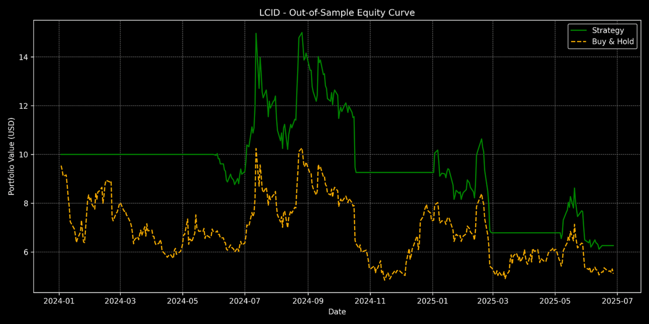
LCID Equity Curve on Testing Data
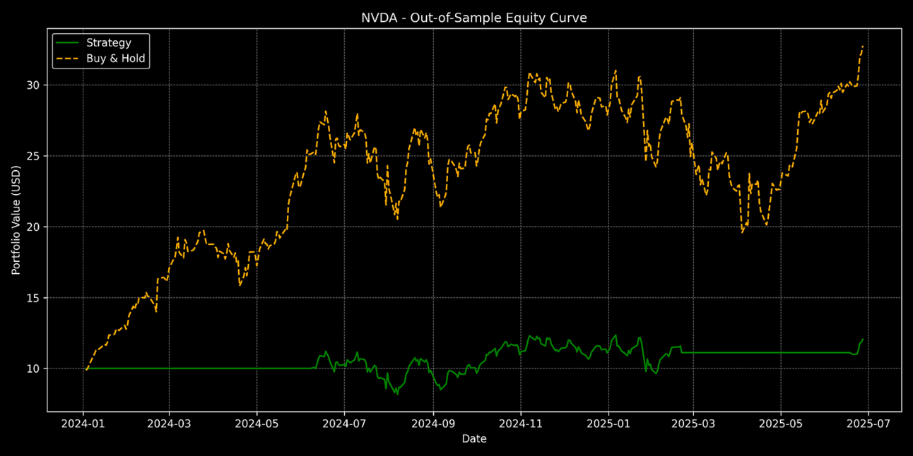
NVDA Equity Curve on Testing Data
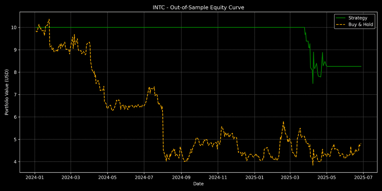
INTC Equity Curve on Testing Data
Compiling and Saving Results for Comparison
After all tickers were processed, I compiled the results into a DataFrame for easy comparison, sorted it by strategy return, saved the summary as a CSV file, and displayed the table for review.
results_df = pd.DataFrame(results)
results_df = results_df.set_index("Symbol")
results_df = results_df.sort_values("Strategy Return (%)", ascending=False)
results_df.to_csv("multi_ticker_strategy_comparison.csv")
results_df
Results of Strategy vs Buy & Hold
Visualizing Comparative Performance
Finally, I visualized the comparative performance by plotting a grouped bar chart showing the return percentages of the optimized strategy versus Buy & Hold for each stock.
This helped identify which tickers benefited most from the strategy.
plt.figure(figsize=(12, 6))
x = np.arange(len(results_df))
width = 0.35

bars1 = plt.bar(x - width/2, results_df["Strategy Return (%)"], width, label="Strategy", color='red')
bars2 = plt.bar(x + width/2, results_df["Buy & Hold Return (%)"], width, label="Buy & Hold", color='green')

for bars in [bars1, bars2]:
    for bar in bars:
        height = bar.get_height()
        plt.text(bar.get_x() + bar.get_width()/2, height + np.sign(height)*2, f"{height:.1f}%",
                 ha='center', va='bottom' if height >= 0 else 'top', fontsize=12)

plt.xticks(x, results_df.index, rotation=45)
plt.ylabel("Return (%)")
plt.title("Strategy vs Buy & Hold Performance (Test Set)")
plt.legend()
plt.grid(True, linestyle='--', alpha=0.5)
plt.tight_layout()
plt.savefig("comparison_bar_chart.png", dpi=300)
plt.show()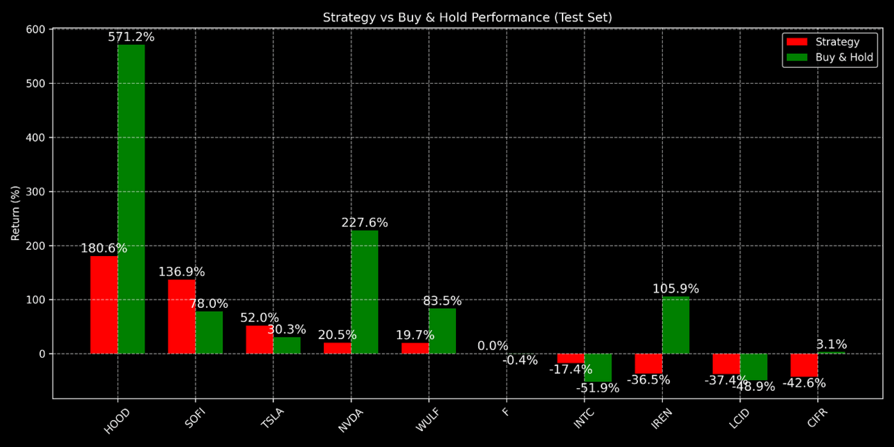
Strategy vs Buy & Hold Performance
Performance Breakdown
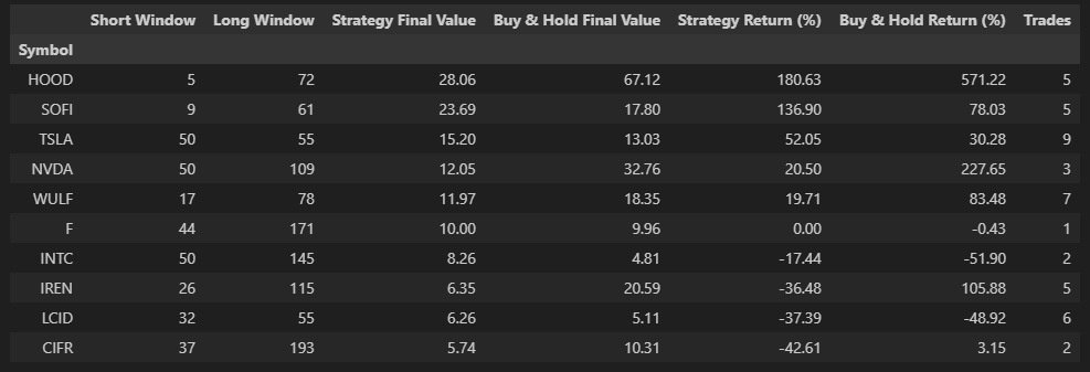
Results of Strategy vs Buy & Hold
I compiled the final returns and number of trades for each stock during the test period. The results revealed some interesting patterns.
For example, the strategy delivered impressive gains on HOOD and SOFI, generating returns of over 130%, while Buy & Hold returns were mixed — extremely high for HOOD but lower for SOFI.
TSLA and WULF also benefited from the strategy, showing double-digit positive returns that in some cases outperformed Buy & Hold.
On the other hand, NVDA had a strong Buy & Hold return of over 227%, while the strategy’s performance was more modest at around 20%.
Some stocks, like INTC, LCID, and CIFR, struggled under the strategy, showing negative returns, though Buy & Hold results varied — INTC and LCID also showed losses with Buy & Hold, while CIFR had a small positive return.
The number of trades varied across stocks, with the strategy typically making fewer than 10 trades during the test period, indicating it was not overly active.
Overall, this comparison helped me understand which tickers responded well to a simple moving average crossover strategy, and which were better suited to passive holding or required more nuanced approaches.
What I Learned
A simple strategy, in the right context, can be surprisingly effective
On fast-moving and highly volatile stocks like HOOD and SOFI, the double moving average crossover strategy managed to capture momentum and ride strong trends.
But on less directional or more erratic stocks, its signals became noisy and less reliable.
Choosing parameters randomly isn’t enough
Using arbitrary moving average windows like 50/200 may work occasionally, but there’s no reason to stick to tradition when we have tools like Bayesian Optimization.
Letting the data guide the parameters gave this simple strategy a real edge during the training phase — and it often carried into the test period.
It’s not about winning everywhere
I didn’t expect this strategy to outperform across the board, and it didn’t. But that wasn’t the point.
The real insight was learning which kinds of stocks respond well to trend-following signals, and which don’t. Buy & Hold is still a solid baseline — but active strategies can have their place, especially when applied with care and context.
Subscribe to our premium content to read the rest.
Become a paying subscriber to get access to this post and other subscriber-only content.
Upgrade


